Vector Databases: Powering Semantic Search and Modern AI Retrieval
Introduction: The Rise of Vector Databases
In today’s AI-driven world, the ability to search and retrieve information based on meaning rather than exact keyword matches has become essential. Enter vector databases—specialized systems designed to efficiently store, index, and query high-dimensional vector representations (embeddings) that capture semantic meaning.
Traditional relational databases excel at structured data queries but falter when asked to find conceptually similar items. They simply weren’t designed for questions like “Find the 10 most semantically similar documents to this text” or “Show me images visually similar to this one.” Vector databases fill this critical gap in our data infrastructure.
These specialized systems are optimized for:
- Efficient nearest neighbor search in high-dimensional spaces
- Scalable embedding storage and retrieval for millions or billions of vectors
- Support for various distance metrics including Euclidean (L2), cosine similarity, and dot product
- Complex semantic queries that go beyond keyword matching
This article explores how vector databases work under the hood, why they’ve become indispensable for modern AI applications, and how they enable cutting-edge technologies like Retrieval-Augmented Generation (RAG).
Understanding Vector Embeddings: The Foundation
Before diving into vector databases, it’s crucial to understand embeddings — the mathematical foundation upon which these systems operate.
What Are Embeddings?
Embeddings are dense numerical representations that capture semantic meaning in a multi-dimensional space. Unlike sparse one-hot encodings, embeddings place semantically similar items closer together in vector space.
When you use models like BERT, GPT, CLIP, or other neural networks, they transform raw inputs (text, images, audio) into these vector representations—typically ranging from 128 to thousands of dimensions. For example:
- BERT base models produce 768-dimensional vectors
- OpenAI’s text-embedding-ada-002 creates 1536-dimensional embeddings
- Many image encoders generate 512 or 1024-dimensional vectors
These embeddings encapsulate rich semantic information that enables similarity-based retrieval. Words like “king” and “queen” end up close to each other in embedding space because they share semantic properties, despite having no character overlap.
Why Store Embeddings?
Generating embeddings is computationally expensive. For applications that need to perform similarity searches over large datasets, it’s impractical to re-generate embeddings for every query. Instead, we:
- Pre-compute embeddings for our corpus (documents, images, products, etc.)
- Store these embeddings in a vector database
- Generate embeddings only for new queries
- Search the database for nearest neighbors to the query embedding
This approach enables sub-second semantic search over massive datasets.
The Anatomy of Vector Databases
Core Components
A vector database typically consists of:
- Vector storage layer: Efficiently stores high-dimensional vectors
- Indexing structures: Enable fast approximate nearest neighbor search
- Metadata storage: Associates vectors with their source data and attributes
- Query interface: Accepts vector similarity queries with filters and parameters
Unlike relational databases with their tables, rows, and columns, vector databases organize data around vectors and the semantic relationships between them.
Distance Metrics: Measuring Similarity
The heart of any vector database is its ability to calculate similarity between vectors. This requires choosing an appropriate distance metric—a mathematical function that quantifies how “far apart” two vectors are. The most common metrics include:
1. Euclidean Distance (L2 Norm)
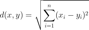
Euclidean distance measures the straight-line distance between vectors, treating the embedding space as a physical space. It’s useful when:
– The absolute position in embedding space matters
– Vectors are normalized to the same magnitude
– The model was specifically trained using L2 distance
2. Cosine Similarity
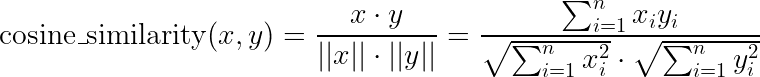
Cosine similarity measures the angle between vectors, ignoring their magnitude. It’s particularly useful for:
– Text embeddings where direction is more important than magnitude
– Comparing documents of different lengths
– Applications where vector magnitude might be influenced by irrelevant factors
3. Dot Product

The dot product combines aspects of both direction and magnitude. It’s useful when:
– Vector magnitude conveys meaningful information
– The model was trained using dot product similarity
– Working with embeddings from attention mechanisms
Choosing the right metric is crucial and depends on how your embeddings were generated and what “similarity” means in your specific context. For general language embeddings, cosine similarity is often the default choice, but experimenting with different metrics can sometimes yield surprising improvements.
Understanding Dimensionality
The dimension of embeddings significantly impacts both storage requirements and query performance. While higher dimensions can theoretically capture more nuanced relationships, they also introduce challenges:

- Storage overhead: Higher dimensions require more bytes per vector
- Computational complexity: Distance calculations become more expensive
- The curse of dimensionality: As dimensions increase, vectors tend to become equidistant from each other
Some vector databases offer dimensionality reduction techniques or specialized storage formats to mitigate these issues. However, it’s important to understand that excessive dimension reduction can destroy the semantic information encoded in the vectors.
Indexing: The Key to Scalable Vector Search
Raw vector storage alone isn’t enough for practical applications. Without efficient indexing, finding nearest neighbors would require comparing a query vector to every vector in the database—prohibitively expensive for large collections.
Indexing Strategies
Vector databases implement various indexing strategies to achieve sub-linear search times:
1. Flat Index (Brute Force)
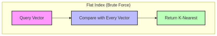
The simplest approach stores vectors without special indexing structures, comparing query vectors against every stored vector.
Pros:
– 100% accurate (returns exact nearest neighbors)
– Simple implementation
– Works well for small datasets (thousands of vectors)
Cons:
– Search time scales linearly with dataset size
– Becomes prohibitively slow for millions of vectors
2. Inverted File Index (IVF)

IVF partitions the vector space into clusters (often using k-means), allowing queries to focus only on relevant partitions:
- During indexing: Vectors are assigned to their nearest cluster centroid
- During querying: The system identifies the closest centroids to the query, then searches only within those clusters
Pros:
– Significantly faster than flat index for large datasets
– Reasonable memory usage – Simple to understand and implement
Cons:
– Accuracy depends on the number of clusters probed
– Requires careful tuning of hyperparameters
– May struggle with high-dimensional data
3. Hierarchical Navigable Small World (HNSW)

HNSW constructs a multi-layered graph where:
– Each vector is a node
– Edges connect similar vectors
– Upper layers form a sparse “express network” for initial navigation
– Lower layers provide more detailed connections
Queries traverse this graph efficiently:
1. Start at entry points in the top layer
2. Greedily move toward closer vectors
3. Descend to lower layers for more precise navigation 4. Eventually reach the exact neighborhood of the query
Pros:
– Excellent search performance (often sub-millisecond)
– High accuracy with proper configuration
– Scales well to millions of vectors
Cons:
– Higher memory requirements
– Complex implementation
– Less efficient for dynamic datasets with frequent additions
4. Product Quantization (PQ)

PQ compresses vectors by dividing them into subvectors, then quantizing each subvector separately:
- Split each d-dimensional vector into m subvectors of d/m dimensions
- For each subvector space, create a codebook with k centroids
- Replace each subvector with the index of its nearest centroid
- Store only the indices (significantly reducing memory footprint)
Pros:
– Dramatically reduces memory footprint
– Enables larger datasets to fit in memory
– Distance calculations can be approximated using pre-computed tables
Cons:
– Reduced accuracy due to quantization errors
– More complex implementation
– Requires careful parameter tuning
Comparison of Indexing Methods
| Method | Search Speed | Memory Usage | Accuracy | Build Time | Dynamic Updates |
|---|---|---|---|---|---|
| Flat (Brute Force) | Slow | Low | 100% | None | Excellent |
| IVF | Medium | Medium | Good (tunable) | Medium | Good |
| HNSW | Very Fast | High | Excellent | Slow | Limited |
| PQ | Fast | Very Low | Lower | Medium | Good |
Popular Indexing Libraries
Many vector databases are built on top of specialized libraries:
- FAISS (Facebook AI Similarity Search): A comprehensive library with various index types and optimization techniques
- Annoy (Approximate Nearest Neighbors Oh Yeah): Spotify’s library known for its simplicity and memory efficiency
- ScaNN (Scalable Nearest Neighbors): Google’s library focused on high performance at scale
- NMSLIB/hnswlib: Libraries implementing the HNSW algorithm with various optimizations
Vector Database Query Patterns
Vector databases support several query patterns beyond basic similarity search:
1. k-Nearest Neighbors (k-NN)
The most common query pattern retrieves the k vectors closest to a query vector. For example:
"Find the 10 most similar products to this one based on user behavior embeddings"2. Radius Search
Returns all vectors within a specified distance threshold:
"Find all documents with a similarity above 0.85 to this query"3. Hybrid Search
Combines vector similarity with metadata filtering:
"Find the most similar articles to this query that were published in the last week and belong to the 'technology' category"4. Batch Search
Efficiently processes multiple query vectors at once:
"Compare these 100 query vectors against our product catalog"These query patterns enable a wide range of applications from recommendation systems to semantic search and anomaly detection.
Retrieval-Augmented Generation (RAG): Vector Databases in Action
One of the most impactful applications of vector databases has emerged with the rise of large language models (LLMs): Retrieval-Augmented Generation.
The RAG Pattern
RAG combines the strengths of retrieval systems and generative AI:

- Indexing stage:
- Split documents into chunks of appropriate size
- Generate embeddings for each chunk
- Store embeddings and text in a vector database
- Query stage:
- Embed the user’s query
- Retrieve relevant document chunks from the vector database
- Inject these chunks as context into the prompt for an LLM
- Generate a response grounded in the retrieved information
This approach addresses several limitations of standalone LLMs:
– Knowledge limitations: RAG can access information beyond the model’s training data
– Hallucination reduction: Providing relevant context helps the model ground responses in facts
– Freshness: The knowledge base can be continuously updated without retraining the model
– Attribution: The system can cite sources for the information provided
Advanced RAG Architectures
The basic RAG pattern has evolved into more sophisticated variants:

Multi-Query RAG
Instead of relying on a single query embedding, this approach:
1. Generates multiple query reformulations using an LLM
2. Embeds each reformulation separately
3. Retrieves results for each variant
4. Aggregates and deduplicates the results
This improves recall by capturing different semantic aspects of the query.

Re-Ranking RAG
Two-stage retrieval improves precision:
1. Initial retrieval: Fast embedding-based search retrieves candidate documents (high recall)
2. Re-ranking: A more sophisticated model re-ranks candidates based on relevance (high precision)
This approach balances efficiency and accuracy, particularly for complex queries.
Self-Querying RAG
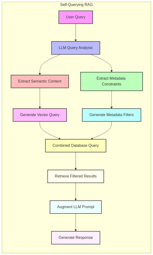
This pattern leverages LLMs to:
1. Analyze the user query to identify both semantic content and metadata constraints
2. Generate appropriate vector search queries and metadata filters
3. Execute the search against a vector database
4. Use the results to produce a comprehensive response
For example, from “Show me articles about renewable energy from the last month,” the system would extract both the semantic query (“renewable energy”) and the metadata filter (publication date).
Real-World Applications
Vector databases enable a wide range of applications:
1. Semantic Search
Unlike keyword search, semantic search understands intent and context:
– E-commerce: “Show me summer dresses with floral patterns” finds relevant products even if they don’t contain those exact words
– Knowledge bases: “How do I troubleshoot slow performance?” returns relevant articles based on meaning, not just keyword matches
2. Recommendation Systems
Vector similarity drives personalized recommendations:
– Content platforms: “Users who enjoyed this content also liked…”
– E-commerce: “Similar products you might be interested in…”
– Media: “Based on your listening history, we recommend…”
3. Anomaly Detection
By embedding normal behavior patterns, systems can identify outliers:
– Fraud detection: Unusual transaction patterns trigger alerts
– Security: Abnormal network traffic or user behavior raises flags
– Manufacturing: Deviations from normal sensor readings indicate potential issues
4. Multi-Modal Search
Vector databases enable cross-modal retrieval:
– Text-to-image: “Find images of a sunset over mountains”
– Image-to-text: “Find articles describing scenes like this image”
– Audio-to-text: “Find transcripts similar to this audio clip”
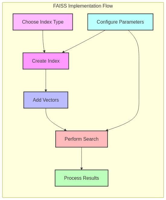
Implementation Example: FAISS in Action
Let’s examine a practical example using FAISS, one of the most popular vector search libraries:
import faiss
import numpy as np

# Configuration
vector_dimension = 128
num_vectors = 100000
k = 5  # Number of nearest neighbors to retrieve

# Generate sample embeddings (in practice, these would come from your ML model)
np.random.seed(42)
database_vectors = np.random.random((num_vectors, vector_dimension)).astype('float32')
query_vector = np.random.random((1, vector_dimension)).astype('float32')

# 1. Create a simple flat index (exact search)
flat_index = faiss.IndexFlatL2(vector_dimension)  # L2 distance
flat_index.add(database_vectors)  # Add vectors to the index

# Search with the flat index
flat_distances, flat_indices = flat_index.search(query_vector, k)
print(f"Flat index results - indices: {flat_indices[0]}, distances: {flat_distances[0]}")

# 2. Create an IVF index (approximate search)
nlist = 100  # Number of clusters
quantizer = faiss.IndexFlatL2(vector_dimension)
ivf_index = faiss.IndexIVFFlat(quantizer, vector_dimension, nlist, faiss.METRIC_L2)

# IVF indices must be trained on a representative dataset
ivf_index.train(database_vectors)
ivf_index.add(database_vectors)

# By default, IVF only searches a subset of clusters
ivf_index.nprobe = 10  # Number of clusters to visit during search

# Search with the IVF index
ivf_distances, ivf_indices = ivf_index.search(query_vector, k)
print(f"IVF index results - indices: {ivf_indices[0]}, distances: {ivf_distances[0]}")
This example demonstrates both exact (flat) and approximate (IVF) search. In practice, you’d:
- Choose an index type based on your dataset size, performance requirements, and accuracy needs
- Carefully tune parameters like
nlistandnprobefor optimal performance - Integrate with a complete vector database solution that handles metadata, persistence, and other features
Challenges and Considerations
1. Scale and Performance
As datasets grow to billions of vectors, challenges arise:
– Memory constraints: High-dimensional vectors consume significant RAM
– Indexing time: Building advanced indexes can take hours for large datasets
– Update frequency: Some index structures require costly rebuilds when adding data
2. Accuracy vs. Speed Tradeoffs
Approximate nearest neighbor algorithms sacrifice some accuracy for speed:
– Recall@k: The percentage of true top-k results that are actually returned
– Query latency: Time to return results, critical for interactive applications
– Index size: Memory footprint of the index structures
Finding the right balance requires careful testing with your specific dataset and use case.
3. Dynamic Data Handling
Many vector databases were initially designed for static datasets:
– Insertion performance: Adding new vectors can be slow for some index types
– Deletion challenges: Some indexes don’t support true deletion without rebuilding
– Reindexing strategies: Periodic rebuilds may be necessary for optimal performance
4. Domain-Specific Considerations
Different domains have unique requirements:
– Text: Handling different languages, document lengths, and semantic nuances
– Images: Managing various resolutions, aspect ratios, and visual features
– Audio: Addressing temporal aspects, variable durations, and audio quality
Future Directions
Vector databases continue to evolve rapidly:
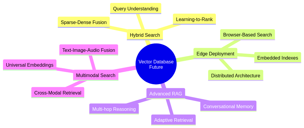
1. Hybrid Search Improvements
Combining vector search with other techniques:
– Sparse-dense fusion: Merging traditional keyword search with embedding-based retrieval
– Learning-to-rank: Using ML to combine multiple relevance signals
– Query understanding: Automatically determining the best search strategy based on query type
2. Edge Deployment
Moving vector search closer to end users:
– Embedded vector indexes: Lightweight implementations for mobile devices
– Browser-based search: WebAssembly implementations of vector search algorithms
– Distributed architectures: Splitting indexes across edge and cloud
3. Advanced RAG Patterns
Evolving beyond basic retrieval:
– Conversational memory: Maintaining context across multiple interactions
– Multi-hop reasoning: Chaining retrievals to answer complex queries
– Adaptive retrieval: Dynamically adjusting retrieval strategies based on query complexity
Conclusion: The Vector-Powered Future
Vector databases have fundamentally changed how we interact with unstructured data. By bridging the gap between raw data and semantic understanding, they’ve enabled a new generation of AI-powered applications that work with meaning rather than just keywords or structured fields.
As foundation models continue to advance, the role of vector databases will only grow in importance. They provide the critical infrastructure layer that allows us to efficiently store, index, and retrieve the semantic representations these models produce.
Whether you’re building a next-generation search engine, a sophisticated recommendation system, or a RAG-powered conversational AI, understanding vector databases is no longer optional — it’s essential knowledge for working in the modern AI landscape.
By mastering these systems, you’ll be equipped to build applications that truly understand what users are looking for, not just what they literally say.