Introduction: The Rise of Vector Databases
We’re drowning in data, yet often starving for meaning. In this AI-inflected era, the crude instruments of keyword search feel increasingly archaic. The ability to retrieve information based on semantic similarity, on intent, isn’t a luxury anymore; it’s the table stakes. Vector databases crash this party – specialized systems forged to tame the wilderness of high-dimensional vector representations, the embeddings that capture meaning itself.
Relational databases, the workhorses of yesteryear, choke on ambiguity. They excel at structured queries but are fundamentally blind when asked to find conceptually similar items. “Find documents like this one”? “Show me images that feel similar”? These questions baffle architectures built on rigid schemas and exact matches. Their very design is orthogonal to the fuzziness, the richness, of semantic space.
Vector databases muscle into this void. They are purpose-built, optimized for the brutal calculus of:
- Efficient nearest neighbor search in the dizzying expanse of high-dimensional spaces.
- Scalable storage and retrieval, handling millions, even billions, of these vector ghosts.
- Support for the right yardsticks: Euclidean distance, cosine similarity, dot product – choosing how you measure “close”.
- Complex semantic queries that leave primitive keyword matching in the dust.
This piece dissects how these databases work under the hood, why they’ve become the indispensable plumbing for modern AI, and how they fuel technologies like Retrieval-Augmented Generation (RAG), dragging language models back towards grounding reality.
Understanding Vector Embeddings: The Foundation
Understand embeddings, or you understand nothing of this domain. They are the bedrock.
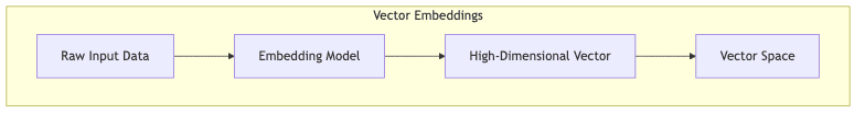
What Are Embeddings?
Embeddings are more than just data; they’re data imbued with meaning. Think of them as dense numerical coordinates pinpointing concepts in a vast, multi-dimensional ‘meaning space’. Unlike sparse, clumsy one-hot encodings, embeddings cluster semantically related items together. Proximity is relevance.
Models like BERT, GPT, CLIP – the modern titans of AI – are embedding factories. They ingest raw stuff (text, images, audio) and transmute it into these vector representations. Typically, these vectors swim in spaces of 128 to thousands of dimensions.
- BERT base models cough up 768-dimensional vectors.
- OpenAI’s
text-embedding-ada-002operates in 1536 dimensions. - Image encoders often settle for 512 or 1024 dimensions.
These aren’t random numbers; they encapsulate semantic relationships. “King” and “Queen” land near each other not because of shared letters, but because of shared meaning. This is the magic we need to harness.
Why Store Embeddings?
Forging these embeddings? Brutally expensive, computationally speaking. Re-generating them on the fly for every query across a large dataset? Insanity. The only sane approach involves pre-computation and storage:
- Pre-compute embeddings for your entire corpus (documents, images, products, user profiles – whatever matters).
- Store these precious vectors in a dedicated vector database.
- Generate embeddings only for the new query as it arrives.
- Search the database, asking it to find the stored vectors closest to your query vector.
This workflow unlocks sub-second semantic search over potentially colossal datasets. It’s the pragmatic path.
The Anatomy of Vector Databases
Core Components
Strip one down, and you’ll typically find:
- Vector storage layer: The vault designed for these high-dimensional numerical ghosts.
- Indexing structures: The clever algorithms enabling fast approximate nearest neighbor search, avoiding brute-force comparisons.
- Metadata storage: The link back to reality, associating vectors with their source data (the document ID, image URL, product SKU) and any filterable attributes.
- Query interface: The front door, accepting similarity queries, filters, and parameters.
Forget tables, rows, and columns. The organizing principles here are vectors and their proximity in meaning space.
Distance Metrics: Measuring Similarity
The soul of a vector database lies in its ability to quantify similarity. This demands choosing the right mathematical yardstick – the distance metric. How “far apart” are two points in this meaning space? Common choices include:
1. Euclidean Distance (L2 Norm)
The straight-line distance. Simple, intuitive, treating the embedding space like physical space. Use it when:
- Absolute position matters.
- Vectors are nicely normalized.
- The embedding model was explicitly trained with L2 in mind.
2. Cosine Similarity
Measures the angle, ignoring vector length (magnitude). King for:
- Text embeddings, where direction often trumps magnitude.
- Comparing items of varying ‘size’ (like short vs. long documents).
- When magnitude might be skewed by irrelevant factors.
3. Dot Product
A blend, sensitive to both direction and magnitude. Useful if:
- Vector magnitude carries real signal.
- The model expects it (common in recommendation systems or attention mechanisms).
Choosing the right metric isn’t academic; it’s fundamental. Pick wrong, and your “similar” results become nonsensical noise. Cosine similarity is often the default for language, but don’t be afraid to experiment; the optimal choice is tied to your specific embeddings and definition of similarity.
Understanding Dimensionality
The number of dimensions in your embeddings is a double-edged sword. It dictates storage costs and query speed. Higher dimensions can capture finer nuances, but they bring the pain:
- Storage Bloat: More dimensions = more bytes per vector. Obvious, but painful at scale.
- Computational Cost: Calculating distances gets heavier.
- The Curse of Dimensionality: In very high dimensions, everything starts looking equidistant – the very notion of “nearest” neighbor frays.
Some databases offer tricks like dimensionality reduction, but wield them carefully. Aggressively compressing vectors can obliterate the subtle semantic information you worked so hard to capture. There’s no free lunch in high dimensions.
Indexing: The Key to Scalable Vector Search
Raw storage is a dead end at scale. Finding nearest neighbors without an index means a brute-force comparison of your query against every single vector in the database. This guarantees glacial performance for any non-trivial dataset. Indexing is the necessary magic.
Indexing Strategies
Vector databases employ clever strategies to achieve sub-linear search times, usually trading a sliver of accuracy for massive speed gains.
1. Flat Index (Brute Force)
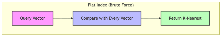
The honest, simpleton approach. Store vectors raw, compare everything.
Pros:
- Perfect accuracy (exact nearest neighbors). Guaranteed.
- Dead simple.
- Fine for tiny datasets (think thousands, maybe low tens of thousands).
Cons:
- Search time scales linearly. O(N). Unworkable for millions/billions.
2. Inverted File Index (IVF)
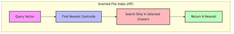
Carve up the meaning space. Partition vectors into clusters (via k-means, usually). Queries only check relevant clusters.
- Index time: Assign each vector to its nearest cluster centroid.
- Query time: Find centroids near the query, search only vectors in those clusters.
Pros:
- Massive speedup over flat for large datasets.
- Memory usage is reasonable.
- Conceptually straightforward.
Cons:
- Approximate. Accuracy depends on how many clusters (
nprobe) you check. - Requires tuning. Getting cluster count and
nproberight matters. - Can struggle with very high dimensions or uneven data distributions.
3. Hierarchical Navigable Small World (HNSW)

The sophisticated graph navigator. Builds a multi-layered graph where vectors are nodes and edges link similar vectors. Upper layers act like highways for coarse navigation, lower layers provide fine-grained connections.
Queries traverse this graph efficiently:
- Enter at sparse top-layer nodes.
- Greedily hop towards vectors closer to the query.
- Drop down layers for more precision.
- Zero in on the nearest neighborhood.
Pros:
- State-of-the-art search speed (often sub-millisecond).
- Excellent accuracy when tuned well.
- Scales gracefully to large datasets.
Cons:
- Memory hungry. The graph structure takes space.
- Complex under the hood.
- Less ideal for datasets with very frequent additions/deletions (can require rebuilds/rebalancing).
4. Product Quantization (PQ)

The memory miser’s trick. Compresses vectors aggressively.
- Chop each vector into smaller subvectors.
- For each subvector position, learn a separate codebook (set of centroids).
- Replace each subvector with the ID of its nearest centroid in its codebook.
- Store sequences of centroid IDs instead of floats.
Pros:
- Massive memory reduction. Fit more vectors in RAM.
- Approximate distance calculations become very fast using pre-computed tables.
Cons:
- Accuracy hit due to quantization (information loss).
- More complex setup and tuning.
Comparison of Indexing Methods
| Method | Search Speed | Memory Usage | Accuracy | Build Time | Dynamic Updates |
|---|---|---|---|---|---|
| Flat (Brute Force) | Slow | Low | 100% (Exact) | None | Excellent |
| IVF | Medium | Medium | Good (tunable) | Medium | Good |
| HNSW | Very Fast | High | Excellent (tuned) | Slow | Limited |
| PQ | Fast | Very Low | Lower (lossy) | Medium | Good |
Popular Indexing Libraries
Often, vector databases build upon battle-tested open-source libraries. Standing on the shoulders of giants (or clever startups):
- FAISS (Facebook AI Similarity Search): The heavyweight champ. Comprehensive, many index types, highly optimized.
- Annoy (Approximate Nearest Neighbors Oh Yeah): Spotify’s creation. Simple, memory-efficient, good for static indexes.
- ScaNN (Scalable Nearest Neighbors): Google’s contender. Focuses on raw performance and accuracy at scale, often using quantization.
- NMSLIB/hnswlib: Popular, high-performance implementations of the HNSW algorithm.
Vector Database Query Patterns
Beyond just finding the closest match, these databases support nuanced queries. Think of them as the verbs of semantic interaction:
1. k-Nearest Neighbors (k-NN)
The bread and butter. Retrieve the k vectors most similar to a query vector. "Find the 10 products semantically closest to this one based on description embeddings"
2. Radius Search
Fetch all vectors within a certain similarity threshold. "Retrieve all news articles published today with a cosine similarity > 0.9 to this breaking event"
3. Hybrid Search
The pragmatic blend. Combine semantic similarity with traditional metadata filtering. "Find the most similar code snippets to this query, but only those written in Python and tagged with 'optimization'"
4. Batch Search
Efficiency play. Process a batch of query vectors simultaneously against the index. "For these 100 user profiles, find their top 5 recommended articles based on viewing history embeddings"
These patterns unlock applications from recommendation engines to semantic search, anomaly detection, and beyond.
Retrieval-Augmented Generation (RAG): Vector Databases in Action
RAG: Where vector databases truly earn their keep. This pattern emerged as a critical patch for the flaws of Large Language Models (LLMs), making vector DBs indispensable.
The RAG Pattern
RAG marries the recall power of retrieval with the generative fluency of LLMs:

- Indexing Phase (Offline):
- Chunk up your knowledge corpus (documents, website data, internal wikis).
- Generate embeddings for each chunk.
- Stuff these embeddings (and the corresponding text) into a vector database.
- Query Phase (Online):
- Embed the user’s incoming query.
- Hit the vector database to retrieve the most relevant chunks.
- Inject these retrieved chunks as context directly into the LLM prompt alongside the original query.
- Ask the LLM to generate a response, now grounded in the retrieved information.
This elegantly tackles several of the LLM’s Achilles’ heels:
- Knowledge Cutoffs: RAG provides access to information beyond the LLM’s static training data.
- Hallucination: Injecting factual context drastically reduces the model’s tendency to invent ‘facts’.
- Stale Information: The vector database can be updated continuously with fresh data, keeping the knowledge current without costly LLM retraining.
- Lack of Attribution: Responses can cite the specific retrieved documents, providing provenance.
Advanced RAG Architectures
The basic RAG concept is just the starting point. The pursuit of relevance leads down more complex paths:

Multi-Query RAG
Don’t bet on a single query embedding. Instead:
- Use an LLM to brainstorm multiple ways to phrase the user’s query.
- Embed each variant.
- Search the vector DB for each embedding.
- Merge the retrieved results intelligently.
This casts a wider semantic net, improving recall for nuanced queries.

Re-Ranking RAG
A two-stage process for better precision:
- Retrieve: Fast vector search pulls a larger set of candidate documents (optimizing for recall).
- Re-rank: A more sophisticated (often computationally heavier) model, like a cross-encoder, meticulously re-scores these candidates for relevance (optimizing for precision).
Balances speed and accuracy, especially crucial when the cost of irrelevant context is high.
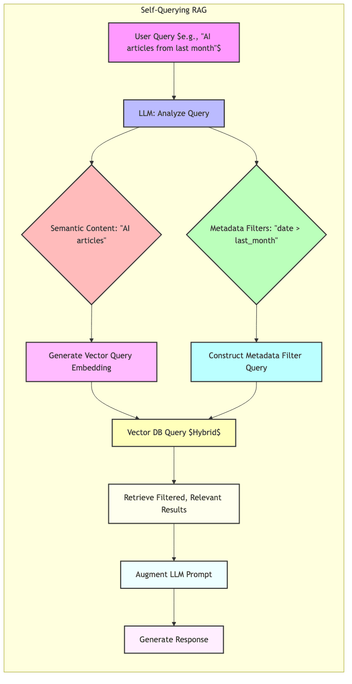
Self-Querying RAG
Use the LLM’s intelligence upfront:
- Let the LLM parse the user query, identifying both the core semantic search terms and any explicit or implicit metadata filters.
- The LLM then constructs the appropriate hybrid query (vector + filters) for the database.
- Execute this structured query.
- Feed the precisely filtered results to the LLM for generation.
Handles complex natural language queries that mix semantic concepts with structured constraints gracefully.
Real-World Applications
The fingerprints of vector databases are all over modern AI applications. The common thread? Moving beyond syntax to semantics.
1. Semantic Search
Understanding intent, not just keywords.
- E-commerce: “Flowery summer dresses” finds relevant products even without those exact terms.
- Knowledge Bases: “Fix slow computer” retrieves meaningful troubleshooting guides.
2. Recommendation Systems
Similarity drives discovery.
- Streaming: “Users who watched X also enjoyed Y…”
- Retail: “Products frequently bought together…” / “Visually similar items…”
- Music: “Because you listened to Z, try this…”
3. Anomaly Detection
Spotting the outliers in embedding space.
- Fraud: Transactions that don’t ‘look like’ normal behavior.
- Security: Network traffic or user actions deviating from the established baseline.
- Industrial IoT: Sensor readings drifting from healthy patterns.
4. Multi-Modal Search
Bridging modalities through shared embedding spaces.
- Text-to-Image: “Generate an image of a cat riding a unicorn.”
- Image-to-Text: “Find articles describing this historical photo.”
- Audio-to-Similar-Audio: “Find podcasts discussing topics similar to this clip.”
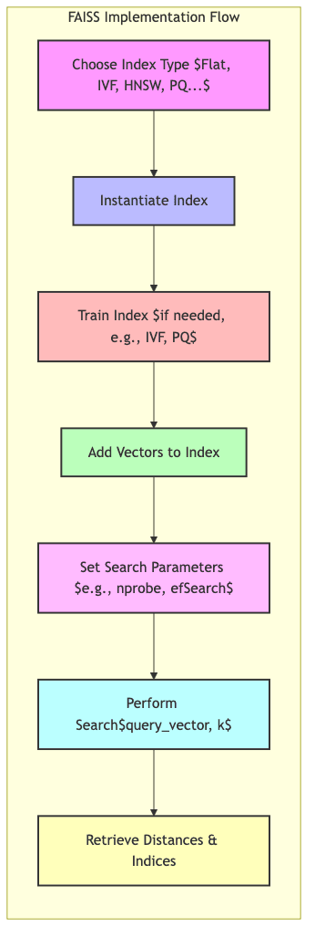
Implementation Example: FAISS in Action
Let’s ground this with a concrete, albeit simplified, example using FAISS:
import faiss
import numpy as np

# Configuration
vector_dimension = 128  # Example dimension
num_vectors = 100000   # Size of our dummy dataset
k = 5                  # How many neighbors we want

# Generate sample embeddings (replace with your actual model outputs)
np.random.seed(42)
database_vectors = np.random.random((num_vectors, vector_dimension)).astype('float32')
query_vector = np.random.random((1, vector_dimension)).astype('float32') # A single query vector

# --- Option 1: Flat Index (Exact Search) ---
print("--- Flat Index (Exact) ---")
flat_index = faiss.IndexFlatL2(vector_dimension)  # Using L2 distance
print(f"Index is trained: {flat_index.is_trained}")
flat_index.add(database_vectors)  # Add all vectors
print(f"Total vectors in index: {flat_index.ntotal}")

# Search the flat index
D_flat, I_flat = flat_index.search(query_vector, k)
print(f"Indices of nearest neighbors: {I_flat[0]}")
print(f"L2 distances: {D_flat[0]}")


# --- Option 2: IVF Index (Approximate Search) ---
print("\n--- IVF Index (Approximate) ---")
nlist = 100  # Number of clusters (cells) to partition data into
quantizer = faiss.IndexFlatL2(vector_dimension)  # Base index for centroids
ivf_index = faiss.IndexIVFFlat(quantizer, vector_dimension, nlist, faiss.METRIC_L2)

# IVF needs training to find the cluster centroids
print(f"Training IVF index...")
ivf_index.train(database_vectors)
print(f"Index is trained: {ivf_index.is_trained}")
ivf_index.add(database_vectors)  # Add vectors, they get assigned to clusters
print(f"Total vectors in index: {ivf_index.ntotal}")

# Tune how many clusters to search (trade-off: speed vs. accuracy)
ivf_index.nprobe = 10  # Search the 10 nearest clusters to the query vector
print(f"nprobe set to: {ivf_index.nprobe}")

# Search the IVF index
D_ivf, I_ivf = ivf_index.search(query_vector, k)
print(f"Indices of nearest neighbors: {I_ivf[0]}")
print(f"L2 distances: {D_ivf[0]}")

# Note: IVF results might differ slightly from Flat due to approximation
This snippet shows the basic flow for both exact (Flat) and approximate (IVF) search with FAISS. In a real application, you’d:
- Select an index type (IVF, HNSW, PQ, combinations thereof) based on scale, performance needs, memory constraints, and accuracy tolerance.
- Meticulously tune index parameters (
nlist,nprobe, HNSW’sMandefConstruction/efSearch, PQ’smandnbits) through experimentation. - Wrap this logic within a complete vector database solution that manages persistence, metadata filtering, APIs, scaling, etc.
Challenges and Considerations
No free lunch here. Vector databases grapple with hard problems:
1. Scale and Performance
Billions of vectors chew through resources:
- Memory Walls: High-dimensional vectors demand substantial RAM, especially for graph-based indexes like HNSW. Disk-based indexes exist but are slower.
- Indexing Time: Building sophisticated indexes on massive datasets isn’t instantaneous; it can take hours or days.
- Update Friction: The messy reality of evolving data. Some indexes (like HNSW) are tricky to update incrementally without performance degradation or costly rebuilds.
2. Accuracy vs. Speed Tradeoffs
The eternal engineering compromise. Approximate Nearest Neighbor (ANN) search is approximate:
- Recall@k: What fraction of the true top-k neighbors did your ANN index actually find? Getting 99% recall might be much slower than 90%.
- Query Latency: Users expect near-instant results. Balancing latency targets with recall is key.
- Index Footprint: Faster, more accurate indexes often consume more memory.
Finding the sweet spot demands rigorous benchmarking on your data and your workload.
3. Dynamic Data Handling
Real-world data isn’t static. Systems must cope with:
- Ingestion Speed: Can the index keep up with new vectors arriving?
- Deletions: True deletions can be notoriously hard in some index structures, often requiring marking-as-deleted and periodic compaction/rebuilds.
- Reindexing Cadence: How often must you rebuild indexes to maintain performance as data shifts?
4. Domain-Specific Nuances
Context matters. Embeddings aren’t one-size-fits-all:
- Text: Multilingual support? Handling variable document lengths effectively during chunking? Semantic subtleties?
- Images: Different resolutions? Aspect ratios? Importance of global vs. local features?
- Audio: Temporal dependencies? Noise robustness? Variable lengths?
Your choice of embedding model, chunking strategy, and distance metric must align with the domain.
Future Directions
The field isn’t standing still; it’s sprinting. Expect continued evolution:
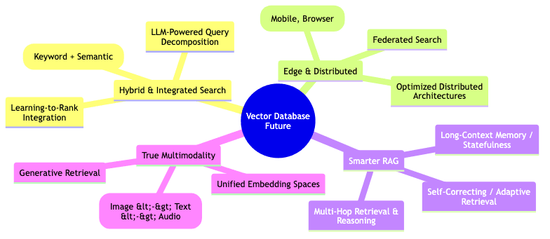
1. Hybrid Search Improvements
Going beyond pure vector similarity:
- Sparse-Dense Fusion: Intelligently combining classic keyword relevance (sparse vectors like BM25) with semantic relevance (dense embeddings).
- Learning-to-Rank (LTR): Using ML models to blend signals from vector similarity, keyword matches, metadata, popularity, etc., into a final ranking.
- LLM Query Understanding: Using LLMs to parse natural language queries and automatically route them to the best strategy (keyword, vector, hybrid, filtered).
2. Edge Deployment
Bringing search closer to the data source:
- Embedded Indexes: Lightweight libraries enabling ANN search directly on mobile devices or in browsers (via WebAssembly).
- Distributed Architectures: Smarter ways to partition and query indexes spread across edge devices and the cloud.
3. Advanced RAG Patterns
Making RAG more robust and intelligent:
- Conversational Memory: Using vector search to give RAG systems persistent memory across turns of a conversation.
- Multi-Hop Reasoning: Architectures that chain multiple retrieval steps to answer complex questions requiring synthesis of information.
- Adaptive Retrieval: Systems that dynamically adjust the number of chunks retrieved or the search strategy based on query complexity or initial results.
Conclusion: The Vector-Powered Future
Vector databases have fundamentally rewired how we grapple with unstructured data. They are the connective tissue between raw information and semantic understanding, the essential infrastructure enabling a new wave of AI applications that operate on meaning, not just syntax.
In the age of foundation models spitting out embeddings for nearly everything, the significance of vector databases only intensifies. They provide the critical layer for storing, indexing, and querying these semantic representations efficiently. Ignoring vector databases is like trying to build a modern web application without understanding HTTP – a recipe for obsolescence.
Whether you’re architecting a search engine that anticipates intent, a recommendation system that intuits taste, or a conversational AI grounded in verifiable facts via RAG, mastering these systems is non-negotiable. It’s the key to building applications that grasp intent, not just keywords, moving us closer to machines that genuinely understand.