1. Introduction: Finding Simplicity in the Chaos
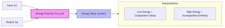
Energy-Based Models (EBMs) aren’t some flashy new invention; they represent a return to fundamental principles, a framework whose elegance is experiencing a resurgence precisely because the field desperately needs it. Forget complex taxonomies of learning methods for a moment. At their heart, EBMs leverage a dead-simple concept: a scalar energy function. This function acts like a universal compatibility meter. Give it a configuration of data, and it spits out a single number – the “energy.”
The rule? Low energy means compatible, likely, or “correct.” High energy means incompatible, unlikely, or “wrong.” That’s it.
While the roots dig deep into statistical physics (think Boltzmann Machines, Hopfield Networks – ghosts of AI past), the current excitement isn’t mere nostalgia. It’s driven by necessity:
- The explosion of self-supervised learning (SSL) demanded a better theoretical underpinning than “it seems to work.”
- Compute finally caught up, making training these models feasible.
- Neural nets became sophisticated enough to actually learn meaningful energy landscapes.
- The relentless push in generative modeling and representation learning needed unifying concepts.
EBMs offer a perspective, a way to think about learning itself. We’ll trace this idea from its core to the clever hacks mitigating its inherent difficulties, showing why this seemingly simple concept holds such profound power.
2. Self-Supervised Learning: Escaping the Label Tyranny
2.1 The Self-Supervision Revolution (or, Reality Bites)
Let’s be blunt: supervised learning, for all its successes, relies on the expensive, often soul-crushing bottleneck of human labeling. Self-supervised learning (SSL) emerged not just as a clever trick, but as a necessary adaptation to a world drowning in unlabeled data yet starved for explicit annotation. It’s about letting the data teach itself, finding the structure hidden within.
Common tactics feel almost like common sense:
- Play hide-and-seek: Mask parts of the data (words, image patches) and make the model guess what’s missing.
- Spot the difference: Teach the model to tell similar things (augmented views of the same image) apart from dissimilar things.
- Clean up the mess: Corrupt the input and train the model to restore the original.
These aren’t just academic exercises; they power giants like BERT, GPT, MAE, and DINO. They proved, decisively, that rich understanding can emerge without someone explicitly telling the model what’s what for every single example.
2.2 EBMs: The Physics Behind Self-Supervision
So, why does SSL work? EBMs offer a compelling answer. Instead of forcing a model to learn a direct mapping (input -> single “correct” output), EBMs focus on learning the compatibility between different pieces of information. The energy function learns the landscape of possibilities.
This shift is more profound than it looks:
- Embraces ambiguity: Real world problems often have multiple valid answers. EBMs don’t have to average them into a blurry mess; they can assign low energy to all good solutions.
- Flexibility: The output doesn’t have to be a single point; it can be a whole region of low energy.
- Rich representations are a side effect: To judge compatibility well, the model must learn meaningful features. Good representations aren’t the goal; they’re a necessary consequence of understanding the energy landscape.
In the EBM view of SSL, the energy function (F(x, y)) measures how well the prediction/completion fits with the context/observed data
. The goal becomes sculpting this energy landscape: pushing down the energy for good pairs and pulling up the energy for bad ones. It’s about learning the rules of the data’s world, not just memorizing input-output pairs.
3. Formal Definition: Giving Structure to the Intuition
3.1 The Scalar Energy Function: The Mathematical Core
Okay, let’s put some mathematical flesh on these bones. An EBM is defined by that scalar function:
Where:
: The stuff you know (input, context, condition).
: The stuff you want to figure out (output, prediction, completion).
: The model’s parameters – the knobs we tune.
- (F(x, y; \theta)): The energy – just a single number telling you how well
fits with
, according to the current model
The core contract remains:
- Low energy: Good fit, compatible, likely.
- High energy: Bad fit, incompatible, unlikely.
Think of this energy as:
- A compatibility score.
- A measure of “surprise” (low energy = unsurprising).
- The negative log-likelihood (if you squint and ignore normalization).
- A learned distance in some abstract feature space.
3.2 From Energy to Probability: The Boltzmann Bridge (and its Pitfalls)
If you absolutely must have probabilities (and sometimes you do), the standard way to link energy to probability is the Boltzmann distribution:
Here, (Z(x; \theta) = \sum_{y’ \in \mathcal{Y}} \exp(-F(x, y’; \theta))) is the infamous partition function. It’s the sum over all possible outputs , ensuring everything adds up to 1. Conceptually neat, practically a nightmare.
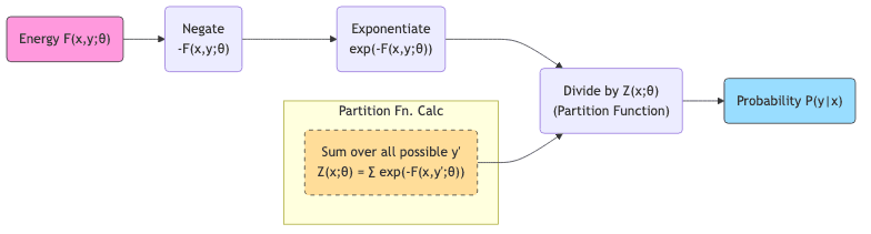
For any interesting problem (images, text, high-dimensional data), calculating (Z(x; \theta)) involves summing over an astronomically large space. It’s computationally intractable. This single hurdle is the mother of invention for most EBM training techniques.
3.3 Training: Dodging the Partition Function
Because calculating directly is usually impossible, we need clever ways to train EBMs without it.
3.3.1 Contrastive Methods: Learning by Comparison
Instead of calculating the full probability distribution, contrastive methods learn by comparing energies. The core idea: make the energy of true data pairs lower than the energy of fake (negative) data pairs, usually by some margin.
[ \mathcal{L}{\text{contrastive}}(\theta) = \mathbb{E}{(x,y_{\text{true}})}\Big[ F(x, y_{\text{true}}; \theta) – \mathbb{E}{y{\text{false}}} [F(x, y_{\text{false}}; \theta)] + \text{margin} \Big]_{+} ]
This family includes Noise Contrastive Estimation (NCE), InfoNCE, and others. The trick lies in generating “good” negative samples that effectively challenge the model.
3.3.2 Score Matching and Denoising: Learning the Landscape’s Slope
Score matching takes a different route. Instead of energy levels, it focuses on the gradient of the log-probability (the “score”). The model learns to predict how the log-probability changes as you tweak the output .
[ \mathcal{L}{\text{score}}(\theta) = \mathbb{E}{(x,y)}\Big[ |\nabla_{y} \log p(y|x) – \nabla_{y} F(x, y; \theta)|^2 \Big] ]
This turns out to be closely related to training models to denoise corrupted data, forming a conceptual link to diffusion models.
3.3.3 Regularization-Based Methods: Preventing Laziness
If you just try to minimize energy for correct pairs, the model might find a trivial solution (like mapping everything to zero energy). Regularization methods add constraints or penalties to force the learned representations to be informative.
Here, (R(\theta)) might encourage high entropy, variance, or decorrelation in the learned features – basically, preventing the model from getting lazy and collapsing its representations. We’ll see specific examples later.
3.4 Inference: Finding the Energy Valleys
Once trained, how do we use an EBM? Usually, we want to find the output that minimizes the energy for a given input
:
Finding this minimum energy state (the “valley” in the energy landscape) can itself be tricky:
- Gradient descent: If
is differentiable w.r.t.
- Sampling: MCMC methods like Langevin dynamics can explore the landscape.
- Amortized inference: Train a separate network to directly predict
.
- Search: For discrete spaces, use search algorithms.
Getting the global minimum isn’t guaranteed; we often settle for a good local minimum.
4. The Value Proposition: Why Bother With All This?
Given the challenges, why embrace EBMs? Because the payoff is significant.
4.1 Advantages: What EBMs Bring to the Table
4.1.1 Handling Reality’s Messiness (Flexibility)
Standard models often struggle when multiple outputs are plausible for one input. They might average possibilities, leading to blurry images or nonsensical text. EBMs excel here. They don’t predict a single ; they evaluate the goodness of any given ((x, y)) pair. This naturally handles ambiguity and complex, multi-modal relationships. Think image completion: an EBM can happily accept many different valid ways to fill in a missing patch, assigning low energy to all of them.
4.1.2 Cutting Through the Jargon (Unified Probabilistic Framework)
EBMs bridge the gap between discriminative models (classifiers) and generative models. The same energy function can be viewed as:
- A compatibility score (discriminative).
- An unnormalized log-probability defining a distribution (generative).
- A mechanism for learning powerful features (representation learning).
This unification helps reveal the common threads running through seemingly different corners of ML.
4.1.3 Building Blocks for Complexity (Compositionality)
Energy functions compose naturally. Want a model that satisfies two different criteria? Just add their energy functions:
This allows for building complex systems from simpler, modular components.
4.2 Challenges: The Dragons We Need to Slay
4.2.1 The Collapse Problem: The Achilles’ Heel
This is the big one, especially for SSL using joint embeddings (where both input and output are mapped to a latent space). The model can discover a trivial “cheat”: map all inputs to the exact same latent vector. If and
are always the same constant, the energy (F(x, y) = |s_x – s_y|^2) is always zero. The loss is minimized, but the model has learned absolutely nothing useful. It’s a catastrophic failure mode.
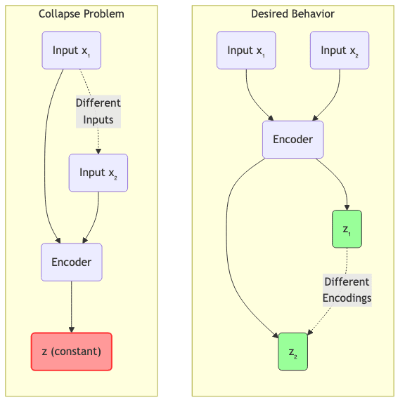
Preventing this collapse is the central theme of many modern EBM/SSL techniques.
4.2.2 Computational Cost: No Free Lunch
Training often requires generating negative samples (expensive) or complex regularization. Inference might involve iterative optimization or sampling. EBMs demand computational resources.
4.2.3 Evaluation: Did It Actually Work?
Measuring the success of an EBM isn’t always straightforward. The partition function is usually unknown, so likelihood is hard to compute. Performance often needs to be assessed indirectly via downstream tasks or proxy metrics that capture representation quality.
5. Modern Approaches: Taming the Collapse Dragon
The need to prevent collapse without resorting to costly negative sampling has spurred incredible innovation.
5.1 The Joint Embedding Framework: Setting the Stage for Collapse
Many modern SSL methods use a joint embedding architecture. Encode the input and target
into latent vectors
and
, then define energy based on their relationship, often simple distance:
As noted, this setup is inherently vulnerable to the trivial collapse solution.
5.2 JEPA: Prediction Creates Asymmetry
Yann LeCun’s Joint Embedding Predictive Architecture (JEPA) introduces a crucial asymmetry: predict the encoding of the target from the encoding of the input.
- Encode context
- Encode target
- Predict
from
: (\hat{s}_y = \text{Pred}(s_x))
- Energy is the prediction error: (F(x, y) = d(\hat{s}_y, s_y))
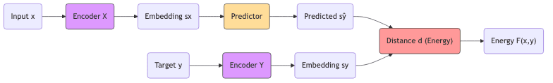
Collapse is avoided because the predictor acts as an information bottleneck, and the target encoder () isn’t directly incentivized to collapse since its output (
) serves as a fixed target for the predictor.
5.3 Non-Contrastive Regularization: Clever Hacks to Avoid Collapse
Several methods achieve collapse prevention through sophisticated regularization, without needing negative samples.
5.3.1 Barlow Twins: Force Decorrelation
Barlow Twins looks at two augmented views () of the same data. It computes their embeddings (
) and then forces the cross-correlation matrix between
and
to be close to the identity matrix.
This means:
- Matching dimensions should be highly correlated (
).
- Different dimensions should be uncorrelated (
). This implicitly prevents collapse by forcing the embedding dimensions to carry diverse information.
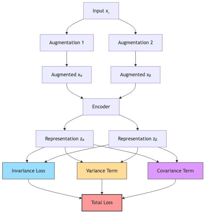
5.3.2 VICReg: Variance, Invariance, Covariance
VICReg (Variance-Invariance-Covariance Regularization) tackles collapse with three simultaneous objectives for embeddings from augmented views:
- Invariance: Make
and
similar (low distance).
- Variance: Keep the variance high along each embedding dimension (prevents collapsing to a point).
- Covariance: Minimize the covariance between different embedding dimensions (encourages decorrelation).
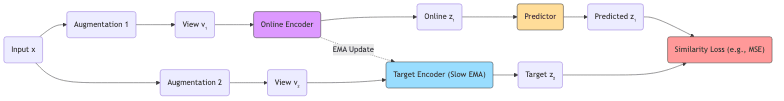
5.3.3 BYOL: Learning from a Slow-Moving Target
BYOL (Bootstrap Your Own Latent) uses an elegant trick involving two networks: an “online” network and a “target” network.
- The online network predicts the target network’s representation of an augmented view.
- The target network’s weights are an exponential moving average (EMA) of the online network’s weights – it changes more slowly.
- This asymmetry – predicting a slightly outdated, stable target – prevents the networks from chasing each other into collapse.
5.4 Cheat Sheet: Ways to Dodge Collapse
| Method | Core Idea | Negative Samples? | Explicit Regularization Focus? |
|---|---|---|---|
| Contrastive | Push true pairs away from fake pairs | Yes | Minimal |
| JEPA | Predict target encoding from context | No | Moderate (via bottleneck) |
| Barlow Twins | Force cross-correlation to identity | No | High (Correlation) |
| VICReg | Maximize variance, minimize covariance | No | High (Statistical) |
| BYOL | Predict slow EMA target network | No | Implicit (Architecture) |
6. A Practical Workflow: Navigating the Implementation Details
Getting EBMs (especially non-contrastive SSL) to work well requires more than just understanding the theory; it involves careful implementation choices.
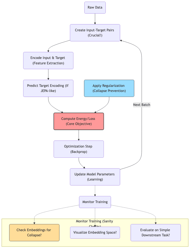
6.1 Data Prep: Garbage In, Garbage Out
The way you structure the learning task is paramount.
- Defining Input/Target: How do you split the data? Masking? Different views? Past/future frames? This defines what compatibility the model learns.
- Augmentation: This is often where the magic (or failure) happens. Augmentations need to be strong enough to challenge the model but shouldn’t destroy essential information. Geometric transforms, color changes, noise, masking – the right mix is domain-specific.
- Batching: Needs care, especially for methods relying on within-batch statistics (like Barlow Twins or VICReg variance terms).
6.2 Architecture: Choosing Your Weapons
The network components matter.
- Encoders: Standard backbones (ResNets, ViTs for vision; Transformers for text) are common starting points. The goal is powerful feature extraction.
- Predictors (if used): Needs careful design. Too simple, and it can’t learn complex relationships. Too complex, and it might overfit or make regularization harder.
- Energy/Similarity Function: Cosine similarity is popular for normalized embeddings; MSE for unnormalized. Sometimes a small learned network (MLP) is used.
6.3 Training: Taming the Beast
Getting the optimization right is often an empirical process.
- Initialization: Can be surprisingly important to avoid immediate collapse.
- Loss Components: Balancing the primary objective (e.g., prediction loss in JEPA) with regularization terms requires tuning hyperparameters (
).
- Optimizer: Adam/AdamW with appropriate learning rate schedules and weight decay are common. Gradient clipping can help stabilize training.
- Monitoring: Essential! Track embedding statistics (variance, std dev across batch) to detect collapse early. Visualize embeddings (t-SNE, UMAP). Periodically evaluate on a simple linear probe task.
6.4 Inference: Using What You’ve Learned
Depends on the goal:
- Prediction/Mapping: Just run the forward pass (encoder + predictor).
- Generation: Requires minimizing the energy function (gradient descent, MCMC) or using a separately trained generator.
- Representation Learning: Throw away everything but the encoder(s) and use them as feature extractors for downstream tasks (fine-tuning or linear probing). This is often the main goal of SSL.
7. Enhanced PyTorch Implementation Sketch
Talk is cheap. Here’s a conceptual PyTorch sketch showing a non-contrastive setup, incorporating ideas reminiscent of VICReg for regularization. (Note: This is illustrative; real implementations require careful tuning and dataset specifics).
import torch
import torch.nn as nn
import torch.optim as optim
import torch.nn.functional as F
from torch.utils.data import DataLoader, Dataset
import torchvision.transforms as transforms

# --- Network Components ---

class EncoderNetwork(nn.Module):
    # Standard MLP encoder with BatchNorm
    def __init__(self, input_dim, latent_dim=256, hidden_dims=[512, 512]):
        super().__init__()
        layers = []
        prev_dim = input_dim
        for h_dim in hidden_dims:
            layers.append(nn.Linear(prev_dim, h_dim))
            layers.append(nn.BatchNorm1d(h_dim)) # BatchNorm is often key
            layers.append(nn.ReLU())
            prev_dim = h_dim
        layers.append(nn.Linear(prev_dim, latent_dim))
        self.encoder = nn.Sequential(*layers)

    def forward(self, x):
        return self.encoder(x.view(x.size(0), -1)) # Flatten input

class PredictorNetwork(nn.Module):
    # MLP predictor for JEPA-style architectures
    def __init__(self, latent_dim, hidden_dim=512):
        super().__init__()
        self.predictor = nn.Sequential(
            nn.Linear(latent_dim, hidden_dim),
            nn.BatchNorm1d(hidden_dim),
            nn.ReLU(),
            nn.Linear(hidden_dim, latent_dim)
        )

    def forward(self, x):
        return self.predictor(x)

class EBM_SSL_Model(nn.Module):
    # Combines encoders and predictor
    def __init__(self, input_dim, latent_dim=256):
        super().__init__()
        # Using same encoder architecture for simplicity, could be different
        self.encoder = EncoderNetwork(input_dim, latent_dim)
        # Might have separate target encoder or use momentum updates (like BYOL)
        # self.target_encoder = EncoderNetwork(input_dim, latent_dim)
        self.predictor = PredictorNetwork(latent_dim) # Only needed for JEPA-like

    def forward(self, x_aug1, x_aug2):
        # Encode both augmented views
        z1 = self.encoder(x_aug1)
        z2 = self.encoder(x_aug2)

        # --- Choose your method's objective ---
        # Example: JEPA-like prediction (predict z2 from z1)
        # z2_pred = self.predictor(z1)
        # return z1, z2, z2_pred

        # Example: Barlow Twins / VICReg (operate directly on z1, z2)
        return z1, z2

# --- Loss Functions ---

# Base energy/similarity - Cosine Similarity often used
def invariance_loss(z1, z2):
    # Normalize embeddings before calculating similarity/distance
    z1_norm = F.normalize(z1, dim=1)
    z2_norm = F.normalize(z2, dim=1)
    # Cosine similarity loss: make similar views have similarity close to 1
    return 2 - 2 * (z1_norm * z2_norm).sum(dim=-1).mean() # Equivalent to MSE on normalized vectors

# VICReg-inspired Regularizers
def variance_loss(z, gamma=1.0, epsilon=1e-4):
    std_dev = torch.sqrt(z.var(dim=0) + epsilon)
    # Penalize std dev falling below gamma
    return F.relu(gamma - std_dev).mean()

def covariance_loss(z):
    n, d = z.shape
    z = z - z.mean(dim=0) # Center features
    cov_matrix = (z.T @ z) / (n - 1)
    # Penalize off-diagonal elements (covariances)
    off_diag_mask = ~torch.eye(d, dtype=torch.bool, device=z.device)
    return (cov_matrix[off_diag_mask] ** 2).sum() / d # Normalize sum

# --- Augmentation & Training Loop ---

# Placeholder for actual data augmentation
class SimpleAugmentation:
    def __call__(self, x):
        # Example: Add noise
        noise = torch.randn_like(x) * 0.05
        return x + noise

def train_ssl_ebm(model, dataloader, optimizer, epochs=100,
                  lambda_inv=1.0, lambda_var=1.0, lambda_cov=0.04): # Lambdas need tuning!

    device = next(model.parameters()).device
    augment = SimpleAugmentation() # Replace with proper augmentations

    for epoch in range(epochs):
        total_loss = 0.0
        model.train()

        for batch in dataloader:
            # Assume batch contains original data samples
            x = batch[0].to(device) # Assuming data comes as (data, label) tuple

            # Create two augmented views
            x_aug1 = augment(x)
            x_aug2 = augment(x)

            # Forward pass (depends on chosen method in model.forward)
            z1, z2 = model(x_aug1, x_aug2)

            # Calculate losses
            inv_loss_val = invariance_loss(z1, z2)
            var_loss_val = variance_loss(z1) + variance_loss(z2) # Apply to both sets of embeddings
            cov_loss_val = covariance_loss(z1) + covariance_loss(z2)

            # Combine losses
            loss = (lambda_inv * inv_loss_val +
                    lambda_var * var_loss_val +
                    lambda_cov * cov_loss_val)

            # Optimization
            optimizer.zero_grad()
            loss.backward()
            optimizer.step()

            total_loss += loss.item()

        avg_loss = total_loss / len(dataloader)
        print(f"Epoch {epoch+1}/{epochs}, Avg Loss: {avg_loss:.4f}")
        # Add monitoring: check std dev of embeddings, etc.

    return model

# --- Main Execution ---
def main():
    # Config
    input_dim = 28 * 28 # MNIST example
    latent_dim = 128
    batch_size = 256
    lr = 1e-3
    epochs = 50

    # Setup - Replace with your actual dataset
    # from torchvision.datasets import MNIST
    # transform = transforms.Compose([transforms.ToTensor()])
    # train_dataset = MNIST(root='./data', train=True, download=True, transform=transform)
    # dataloader = DataLoader(train_dataset, batch_size=batch_size, shuffle=True, num_workers=4)

    # Dummy data for demonstration
    class DummyDataset(Dataset):
        def __init__(self, num_samples=10000, dim=784):
            self.data = torch.randn(num_samples, dim)
        def __len__(self): return len(self.data)
        def __getitem__(self, idx): return self.data[idx], 0 # Return dummy label

    dummy_dataset = DummyDataset()
    dataloader = DataLoader(dummy_dataset, batch_size=batch_size, shuffle=True)

    # Init model and optimizer
    device = torch.device("cuda" if torch.cuda.is_available() else "cpu")
    model = EBM_SSL_Model(input_dim, latent_dim).to(device)
    optimizer = optim.AdamW(model.parameters(), lr=lr, weight_decay=1e-5) # AdamW often preferred

    print(f"Using device: {device}")

    # Train
    trained_model = train_ssl_ebm(model, dataloader, optimizer, epochs)

    print("Training finished.")
    # Now use trained_model.encoder for downstream tasks

if __name__ == "__main__":
    main()
This sketch provides a more concrete structure, including basic regularization terms inspired by VICReg, highlighting the interplay between components. Remember, the devil is in the details: augmentations, hyperparameter tuning (s), and architecture choices are critical.
8. Recent Advances and Future Directions: Where Does the Energy Flow Next?
The EBM perspective isn’t static; it continues to evolve and permeate other areas.
8.1 Merging with Foundation Models
The ideas aren’t just for bespoke SSL models anymore. They’re influencing how we understand and build foundation models:
- LLMs: While trained on next-token prediction, the probability distribution an LLM implicitly models is an energy landscape over sequences. Techniques like contrastive decoding explicitly leverage this.
- Vision-Language: CLIP-style models learn joint embedding spaces where similarity is effectively negative energy. They learn cross-modal compatibility.
- Diffusion Models: These are intimately related to score matching, directly learning the gradient of the log-probability (related to the energy gradient). They are, in essence, a powerful way to train and sample from EBMs.
8.2 Multimodal EBMs: Bridging Senses
EBMs offer a clean way to model compatibility across different data types (text, image, audio, etc.). An energy function (F(x_{\text{text}}, x_{\text{image}}, x_{\text{audio}})) can naturally score how well different modalities align, driving progress in retrieval, generation, and understanding tasks that span multiple senses.
8.3 Blurring Lines: Discriminative vs. Generative
EBMs sit comfortably astride the old divide. They learn representations discriminatively (judging good vs. bad pairs) but implicitly define a generative model (via Boltzmann). This duality fuels research into:
- Better sampling methods to turn EBMs into efficient generators.
- Hybrid models combining EBM strengths with other generative approaches (like GANs or VAEs).
- Transferring knowledge learned discriminatively to generative tasks.
8.4 Reinforcement Learning: Learning What’s Good
In RL, EBMs are emerging as tools for:
- World models: Predicting future states (low energy for plausible futures).
- Reward modeling: Learning energy functions that assign low energy to desirable states/actions, often from demonstrations.
- Hierarchical RL: Representing goals or sub-tasks within an energy framework.
9. Conclusion: It Really Is (Mostly) About Energy
Energy-Based Models, particularly in their modern non-contrastive SSL flavors, aren’t just another technique. They offer a fundamental, unifying perspective on learning complex relationships in data. By shifting focus from direct prediction to compatibility scoring, they elegantly handle ambiguity, promote rich representation learning, and bridge diverse areas of machine learning.
Key Takeaways (RK Remix):
- Simplicity Wins: Underneath the complex architectures and math, the core idea is dead simple: low energy = good fit. This provides a powerful unifying lens.
- Collapse is the Enemy: The biggest practical hurdle was the model finding trivial, useless solutions. Modern SSL is largely about clever ways to prevent this.
- No More Contrast?: Methods like JEPA, VICReg, Barlow Twins, and BYOL show you can often avoid the hassle of explicit negative sampling through smart regularization or architectural design.
- Implementation Matters: Theory is nice, but success lies in careful architecture, strong augmentation, robust regularization, and diligent monitoring.
- The Future is Energetic: EBM concepts are bleeding into foundation models, multimodal learning, and even RL, suggesting their influence will only grow.
As we push towards more autonomous, generalizable AI systems capable of learning from the deluge of unlabeled data, understanding the “physics” of compatibility – the energy landscape – seems increasingly crucial. The EBM framework, combined with the practical ingenuity of recent deep learning advances, provides a powerful pathway forward. It’s not just about building models; it’s about understanding the fundamental principles of how systems can learn the structure of their world.
Further Reading (If you must dig deeper…)
- Yann LeCun, et al. “A Path Towards Autonomous Machine Intelligence” (2022) – The JEPA vision paper.
- Barlow Twins, VICReg, BYOL papers – Details on the clever non-contrastive tricks.
- Score-Based Generative Modeling literature – Connections to diffusion models.
- Du & Mordatch, “How to Train Your Energy-Based Models” (2019) – Practical tips (though somewhat dated now).
- Nijkamp et al., “Implicit Maximum Likelihood Estimation” (2019) – Advanced training/sampling ideas.