Diffusion Models in AI Image Generation – Part 2: Applications & Advancements

Introduction: From Mechanics to Manipulation

In Part 1, we dissected the core mechanics of diffusion models – the structured destruction and reconstruction of information via noise. We saw how they learn to reverse entropy, step-by-step, to synthesize coherent images. Now, we shift focus from the underlying physics to the engineering and application: how do we bend these probabilistic processes to our will, and what tricks have emerged to make them practical tools rather than just theoretical curiosities?

The dominant application, the one consuming most of the oxygen, is text-to-image generation. Systems like DALL·E, Midjourney, and Stable Diffusion didn’t just appear; they rely on layering control mechanisms onto the core diffusion process. The challenge is not just generating an image, but generating the specific image described by a user’s text prompt. This requires sophisticated methods for injecting textual guidance into the denoising loop.

We’ll also examine the critical engineering hacks, like latent diffusion, that wrestled these computationally ravenous models into something usable outside massive research labs. And we’ll look at the ongoing arms race for speed, exemplified by techniques like Latent Consistency Models, pushing towards the still-elusive goal of real-time, high-fidelity generation. Forget the theory for a moment; this is about how the machine is actually built and operated.

Text-to-Image Generation: Steering the Noise

Generating images from pure noise is interesting, but generating images from text is where diffusion models became truly disruptive. This requires imposing external constraints onto the denoising process.

Injecting Conditional Guidance

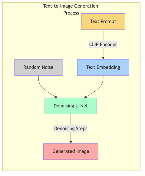
To make the model responsive to a text prompt, we need to condition its behavior. The typical workflow involves:

1. Text Encoding: The input prompt is transformed into a meaningful numerical vector (an embedding) using a separate, pre-trained model, often a variant of CLIP (Contrastive Language–Image Pre-training). This embedding captures the semantic essence of the prompt.
2. Conditioning the Diffusion: This text embedding is fed into the diffusion model (typically a U-Net architecture) alongside the noisy image at each denoising step.
3. Guided Sampling: The model is now tasked with predicting noise not just to create any plausible image, but one that aligns with the provided text embedding.

The U-Net’s objective changes subtly: “Predict the noise removal step that moves this noisy image closer to a clean image consistent with this text description.”

Classifier-Free Guidance: Amplifying the Prompt’s Influence

Simply feeding the text embedding helps, but results can be weak. A more potent technique, classifier-free guidance (CFG), emerged as a standard way to strengthen the prompt’s influence. The core idea is clever:

1. Dual Training: Train the diffusion model to operate in two modes: conditionally (with a text prompt) and unconditionally (receiving a null or empty prompt).
2. Dual Prediction During Inference: At each denoising step, calculate two noise predictions:
   • One based on the noisy image and the actual text prompt ().
   • One based on the noisy image but the null prompt ().
3. Extrapolation: Combine these predictions. The difference between the conditional and unconditional predictions represents the direction the prompt is “pulling” the generation. We can amplify this direction using a guidance scale ():

Here:

• is the noise prediction guided by text prompt .
• is the noise prediction without guidance (the unconditional path).
• is the guidance scale. Higher values (e.g., 7-12) force stricter adherence to the prompt, often at the cost of some naturalness or introducing artifacts. Lower values yield more varied but potentially less relevant results.

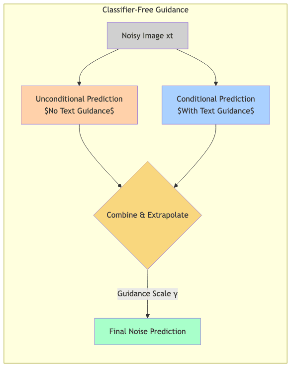
CFG essentially asks: “How would the prediction change if we did consider the prompt?” and then exaggerates that change. It’s a powerful heuristic for trading off creativity against prompt fidelity.

Prompt Engineering: The Necessary Artifice

The blunt instrument of text prompts means that controlling the output often requires careful phrasing – a practice that’s evolved into “prompt engineering.” This involves strategically using keywords and structures to wrestle the desired output from the model:

• Style Injection: “oil painting,” “photorealistic,” “vaporwave,” “cinematic lighting.”
• Artist Mimicry: “in the style of H. R. Giger,” “cinematography by Roger Deakins.”
• Quality/Detail Modifiers: “8K,” “highly detailed,” “sharp focus,” “intricate.”
• Negative Prompts: Defining exclusions (“avoid blurry faces,” “no text,” “not deformed”).

The sophistication (and sometimes absurdity) of prompt engineering highlights the current limitations in our ability to communicate nuanced visual intent directly to these models. It’s a craft born of necessity.

Latent Diffusion: Escaping Pixel Tyranny

Early diffusion models operated directly on pixels. Given the high dimensionality of images (a 512×512 image has 786,432 dimensions if RGB), this was computationally brutal. Latent diffusion provided a crucial optimization by shifting the battlefield to a compressed, lower-dimensional latent space.

The Compression Gambit

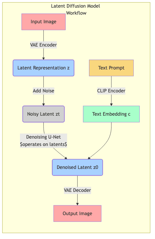
Latent diffusion models leverage a separate autoencoder, usually a Variational Autoencoder (VAE), for dimensionality reduction:

1. Encoder: Compresses a high-resolution image into a much smaller latent representation (e.g., 64x64x4 instead of 512x512x3). This latent vector captures the essential semantic information.
2. Decoder: Reconstructs a full-resolution image from a latent representation.

The entire diffusion process—adding noise and iteratively denoising—occurs within this compact latent space. Only the initial encoding and final decoding steps interact with the pixel space.

Why Latent Space Wins

• Massive Computational Savings: Operating on smaller latent tensors dramatically cuts memory and compute requirements (often by factors of 4x to 8x or more).
• Faster Operations: Training and inference cycles are significantly quicker.
• High-Resolution Feasibility: Generating large images becomes practical because the expensive diffusion happens on small latents.
• Quality Preservation: The VAE is trained to retain perceptual quality, so diffusion in latent space yields results comparable or superior to pixel-space models.

Latent diffusion, popularized by Stable Diffusion, was arguably the key innovation that moved powerful diffusion models from cloud servers onto consumer-grade GPUs.

Accelerating Sampling: The Need for Speed

While latent diffusion drastically reduced the cost per step, the number of steps remained a bottleneck. Early models needed 50, 100, or even more sequential denoising steps for good results, making generation slow. This sparked intense research into reducing this step count.

Latent Consistency Models: Leaping Through Latent Space

Latent Consistency Models (LCMs) emerged as a major breakthrough, slashing the required sampling steps, often down to just 1-8, while largely preserving quality.

What Are LCMs?

LCMs are derived from existing diffusion models via distillation. Their goal is to learn the outcome of multiple diffusion steps directly, enabling much larger jumps through the denoising process. Key characteristics:

• Distilled Models: They learn from a pre-trained “teacher” diffusion model.
• Few-Step Inference: Designed for high-quality output in typically 1 to 8 steps, versus 20-50+ for standard models.
• Quality Retention: Aim to match the parent model’s style and prompt adherence.

The ODE Perspective

Instead of viewing diffusion reversal as a sequence of stochastic steps (adding predicted noise back), LCMs leverage the perspective of solving an underlying Ordinary Differential Equation (ODE). The trajectory from pure noise to a clean image in latent space can be seen as following a path defined by a probability flow ODE.

• LCMs learn to predict points far along this trajectory directly.
• This allows skipping many intermediate steps that traditional samplers would simulate.
• The model effectively learns a shortcut to the solution of the diffusion ODE.

Impact of LCMs

The speedup is not incremental; it’s transformative:

• Enables near real-time image generation on capable hardware.
• Makes interactive editing and generation loops practical.
• Drastically reduces inference costs for services.
• Improves feasibility of diffusion-based video generation (faster frame rendering).

Creating LCMs: Knowledge Distillation

The standard method for creating LCMs is knowledge distillation:

1. Teacher Model: Use a fully trained, high-quality diffusion model.
2. Student Model: Initialize a new model (often with the same architecture).
3. Training Objective: Train the student to predict the result of several teacher steps, or points further along the ODE trajectory, in a single step. The teacher provides the “ground truth” trajectories.
4. Fine-tuning: Refine the student for optimal quality at very low step counts.

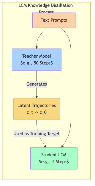
Distillation transfers the learned capabilities of the large teacher into a much faster student optimized for few-step inference.

Alternative Acceleration Paths

LCMs are potent, but other methods also tackle sampling speed:

1. Improved Samplers (Schedulers): Algorithms like DDIM (Denoising Diffusion Implicit Models) offered early deterministic sampling improvements. More advanced solvers like DPM-Solver and DPM-Solver++ treat diffusion as an ODE and employ sophisticated numerical methods to solve it efficiently in fewer steps (e.g., 15-25).
2. Consistency Models: A related concept where models learn to map any point on the noise trajectory directly to the final clean image ().
3. Progressive Distillation: Iteratively distilling models, where a faster student becomes the teacher for an even faster student.

The choice often involves trade-offs between speed, fidelity, sample diversity, and implementation complexity.

Implementation Snapshot: Working with Diffusers

Libraries like Hugging Face’s diffusers abstract away much of the complexity, providing high-level interfaces to various models and techniques.

Baseline: Stable Diffusion Text-to-Image

# Ensure 'diffusers', 'transformers', 'torch', 'accelerate' are installed
import torch
from diffusers import StableDiffusionPipeline

# Load a standard Stable Diffusion model (e.g., v2.1)
model_id = "stabilityai/stable-diffusion-2-1"
# Use float16 for efficiency if GPU supports it
pipe = StableDiffusionPipeline.from_pretrained(model_id, torch_dtype=torch.float16)
pipe = pipe.to("cuda") # Move model to GPU

prompt = "A majestic snow leopard perched on a rocky cliff, detailed fur, hyperrealistic, cinematic lighting"
negative_prompt = "cartoon, drawing, illustration, sketch, blurry, low quality, deformed"

# Generate image using standard parameters
with torch.autocast("cuda"): # Use automatic mixed precision
    image = pipe(
        prompt=prompt,
        negative_prompt=negative_prompt,
        num_inference_steps=30,  # Typical steps for good quality
        guidance_scale=7.5,      # Standard CFG scale
        width=768,               # Example resolution
        height=512
    ).images[0]

image.save("snow_leopard_sd.png")
print("Standard SD image saved.")

Accelerated: Latent Consistency Model (LCM)

import torch
from diffusers import LCMScheduler, AutoPipelineForText2Image

# Load a model compatible with LCM (can be base SD model)
model_id = "stabilityai/stable-diffusion-xl-base-1.0"
pipe = AutoPipelineForText2Image.from_pretrained(model_id, torch_dtype=torch.float16, variant="fp16")

# Configure the pipeline to use the LCM Scheduler
pipe.scheduler = LCMScheduler.from_config(pipe.scheduler.config)
pipe.to("cuda")

# Load LCM LoRA weights specific to the base model
lcm_lora_id = "latent-consistency/lcm-lora-sdxl"
pipe.load_lora_weights(lcm_lora_id)
pipe.fuse_lora() # Optional: fuse LoRA for slightly faster inference

prompt = "Self-portrait oil painting, Van Gogh style, swirling clouds"

# Generate with very few steps
# Note: LCMs often work better with lower guidance or guidance disabled (scale=0)
with torch.autocast("cuda"):
    image = pipe(
        prompt=prompt,
        num_inference_steps=4,    # Drastically fewer steps
        guidance_scale=0,       # Disable CFG for pure LCM speed
        width=1024,
        height=1024
    ).images[0]

image.save("van_gogh_lcm.png")
print("LCM image saved.")

# Unload LoRA weights if you want to use the pipe for other things
# pipe.unfuse_lora()
# pipe.unload_lora_weights()

Optimized Sampling: Using DPM-Solver++

import torch
from diffusers import StableDiffusionPipeline, DPMSolverMultistepScheduler

# Load the base model again
model_id = "stabilityai/stable-diffusion-2-1"
pipe = StableDiffusionPipeline.from_pretrained(model_id, torch_dtype=torch.float16)

# Switch to a more efficient scheduler
pipe.scheduler = DPMSolverMultistepScheduler.from_config(pipe.scheduler.config)
# Recommended DPM++ settings often include Karras sigmas
# pipe.scheduler = DPMSolverMultistepScheduler.from_config(pipe.scheduler.config, use_karras_sigmas=True, algorithm_type="sde-dpmsolver++")

pipe = pipe.to("cuda")

prompt = "Steampunk owl robot, intricate gears, brass and copper, detailed illustration"

# Generate with fewer steps than default, thanks to the scheduler
with torch.autocast("cuda"):
    image = pipe(
        prompt,
        num_inference_steps=20,  # Reduced steps viable with DPM++
        guidance_scale=7.0
    ).images[0]

image.save("steampunk_owl_dpm.png")
print("DPM-Solver++ image saved.")

These examples illustrate how different components—the base model, acceleration techniques (LCM via LoRA), and sampling schedulers—interact to affect speed and quality. The diffusers library provides the building blocks to experiment with these combinations.

Navigating Implementation: Ground Truths

Working effectively with diffusion models involves grappling with their inherent characteristics and limitations.

Image Quality Fundamentals

1. Native Resolution is Key: Models perform best near their training resolution (e.g., 512×512 for SD 1.5, 1024×1024 for SDXL). Straying too far often degrades quality or introduces artifacts like duplication. Upscaling is often a separate post-processing step.
2. Aspect Ratio Sensitivity: While not strictly square, models are sensitive to extreme aspect ratios. Stick to common ratios (16:9, 3:2, 4:3) to avoid warped compositions.
3. Seed Management: A fixed random seed ensures reproducibility. Small variations around a good seed can explore stylistic nuances without changing the core composition. It’s crucial for iterative refinement.
4. Compositional Limits: Complex scenes with multiple interacting subjects remain challenging. Techniques like regional prompting, generating elements separately, or using control nets (like ControlNet for pose/depth) are often needed for precise layout.

Performance Considerations

1. Batching: Generating images in batches leverages GPU parallelism but increases peak memory load. Find the sweet spot for your hardware.
2. Precision: float16 (half-precision) is standard for inference, offering significant speed and memory gains over float32 with negligible quality impact on modern GPUs.
3. Memory Optimization: Techniques like attention slicing or offloading parts of the model to CPU can enable running larger models on constrained hardware, at the cost of speed.
4. Model Loading Overhead: Loading large models into memory takes time. For applications needing responsiveness, keeping models loaded (if feasible) is critical.

Prompting Realities

1. Specificity vs. Exploration: Detailed prompts yield specific results; shorter, vaguer prompts allow the model more creative freedom (and variance).
2. Keyword Weighting Nuances: Syntax like (keyword:1.3) or [keyword] (for negative emphasis in some UIs) helps prioritize terms, but effectiveness varies between models and implementations.
3. The Power of Negation: Negative prompts are essential for cleaning up common failure modes (mangled hands, extra limbs, watermarks, text).
4. Iterative Refinement: Finding the optimal prompt is often a process of trial, error, and adjustment based on generated outputs. Don’t expect perfection on the first try.

Emergent Trajectories: What’s Next?

Diffusion model research continues at a blistering pace. Key frontiers include:

Video Diffusion

Extending the step-by-step generation process to sequences of frames. Models like Sora, Stable Video Diffusion, and others are making progress, but maintaining long-range temporal coherence (consistent object appearance and motion) remains the central challenge.

3D Generation

Applying diffusion principles to generate 3D assets (meshes, textures, NeRFs, point clouds). Challenges include capturing complex geometry, consistent texturing, and generating formats usable in standard 3D workflows.

Personalization and Fine-tuning

Making models adaptable without full retraining. Techniques like DreamBooth (subject replication), LoRA (Low-Rank Adaptation for style/concept tuning), and Textual Inversion (embedding new concepts) allow for efficient customization.

Multimodal Integration

Weaving diffusion models into larger systems that handle multiple data types. This includes generating images based on combined text/image/audio inputs, editing images via natural language commands, or generating audio/video conditioned on text/images.

Conclusion: The Diffusion Engine Evolves

In a remarkably short period, diffusion models have shifted from academic papers to foundational components of the generative AI landscape. Their capacity for high-fidelity image synthesis, combined with increasingly sophisticated control mechanisms like text conditioning and CFG, underpins the current generation of creative tools.

The development of latent diffusion made these models computationally accessible, while the relentless pursuit of faster sampling—spearheaded by techniques like LCMs and advanced ODE solvers—is pushing towards interactive speeds. These engineering efforts are as crucial as the core algorithmic insights.

While challenges remain—true compositional control, temporal consistency in video, robust 3D generation—the trajectory is clear. The fundamental principles of iterative denoising, guided by various conditioning signals and optimized through clever engineering, provide a powerful and flexible framework. Understanding these mechanics, from noise schedules to latent spaces to CFG, is key to harnessing current tools and anticipating the next wave of innovation in generative AI. The process of refining noise into signal continues, getting faster and more controllable with each iteration.