Vision Transformers: How “An Image is Worth 16×16 Words”
Introduction
When Transformers revolutionized natural language processing starting in 2017, many researchers wondered: could the same architecture work for computer vision? The answer came in 2020 with the publication of “An Image is Worth 16×16 Words” by Dosovitskiy et al. from Google Research, introducing the Vision Transformer (ViT).
ViT challenged the long-standing dominance of Convolutional Neural Networks (CNNs) in computer vision by demonstrating that a pure Transformer architecture—with minimal domain-specific modifications—could achieve state-of-the-art results on image classification tasks. This would obviously pave way for Multimodal models with Transformers now powering many cutting-edge vision systems.
In this article, we’ll explore:
- The key insights behind Vision Transformers,
- A detailed breakdown of the ViT architecture,
- How ViTs compare to CNNs across different data regimes,
- Recent advancements and practical applications, and
- Implementation considerations for researchers and practitioners.
The Paper at a Glance
- Title: “An Image is Worth 16×16 Words: Transformers for Image Recognition at Scale” (2020)
- Authors: Alexey Dosovitskiy, Lucas Beyer, Alexander Kolesnikov, et al. (Google Research, Brain Team)
- Key Innovation: Applying the Transformer architecture directly to images by treating non-overlapping image patches as “tokens” (similar to words in NLP).
- Model Architecture: An encoder-only Transformer that processes a sequence of image patches plus a special learnable “class token”.
- Performance: When pre-trained on large datasets (14M-300M images), ViT outperformed state-of-the-art CNNs while requiring fewer computational resources to train.
The ViT Architecture: A Closer Look
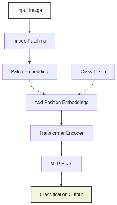
Image-to-Sequence Conversion: Patch Embedding
The first innovation of ViT lies in how it transforms an image into a sequence:
- Image Patching: The input image (typically 224×224 pixels) is divided into fixed-size non-overlapping patches (e.g., 16×16 pixels), resulting in a grid of patches (14×14 for a 224×224 image with 16×16 patches).
- Patch Flattening: Each patch is flattened into a 1D vector. For a 16×16 patch with 3 color channels, this results in a 768-dimensional vector (16 × 16 × 3 = 768).
- Linear Projection: Each flattened patch is projected to the model’s embedding dimension (e.g., 768) using a trainable linear projection.

This process effectively converts a 2D image into a 1D sequence of patch embeddings, similar to how words are embedded in NLP Transformers.
Here’s a simplified implementation of the patch embedding process:
import torch
import torch.nn as nn

class PatchEmbedding(nn.Module):
    def __init__(self, img_size=224, patch_size=16, in_chans=3, emb_dim=768):
        super().__init__()
        self.img_size = img_size
        self.patch_size = patch_size
        self.num_patches = (img_size // patch_size) ** 2
        # Implementation using Conv2d with kernel_size=stride=patch_size
        # This efficiently performs both patch extraction and linear embedding
        self.proj = nn.Conv2d(in_chans, emb_dim, kernel_size=patch_size, stride=patch_size)

    def forward(self, x):
        # x shape: (batch_size, channels, height, width)
        B, C, H, W = x.shape
        assert H == W == self.img_size, f"Input image size ({H}*{W}) doesn't match expected size ({self.img_size}*{self.img_size})"

        x = self.proj(x)  # shape: (batch_size, emb_dim, grid_height, grid_width)
        x = x.flatten(2)  # shape: (batch_size, emb_dim, num_patches)
        x = x.transpose(1, 2)  # shape: (batch_size, num_patches, emb_dim)
        return x
Position Information and Class Token
Unlike CNNs, Transformers have no inherent understanding of spatial relationships. ViT addresses this limitation with two key elements:
1. Positional Embeddings
To give the model information about the spatial arrangement of patches, ViT adds learnable 1D positional embeddings to each patch embedding. These embeddings encode the position of each patch in the original 2D grid, allowing the model to reason about spatial relationships.
2. Class Token
Inspired by BERT’s [CLS] token, ViT prepends a special learnable “class token” to the sequence of patch embeddings. After processing through the encoder, the final representation of this class token serves as the image representation for classification.
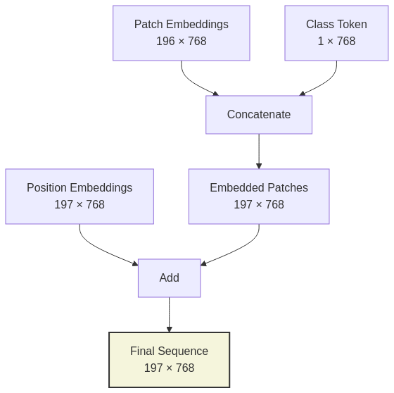
Transformer Encoder
After obtaining the final sequence of embeddings (patch embeddings + class token + positional embeddings), ViT processes this sequence through a standard Transformer encoder consisting of:
- Multi-Head Self-Attention (MSA): Allows each patch to attend to other patches, capturing both local and global dependencies.
- Multi-Layer Perceptron (MLP): A two-layer feed-forward network with GELU activation.
- Layer Normalization and Residual Connections: Applied before each block (pre-norm formulation).

As you might already know, the self-attention mechanism can be expressed mathematically as:
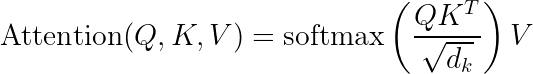
Where  ,
,  , and
, and  are the query, key, and value matrices, and
  is the dimension of the key vectors.
The multi-head attention extends this by computing attention multiple times in parallel:


Here’s a more complete implementation including the transformer encoder and full model:
class TransformerEncoder(nn.Module):
   def __init__(self, emb_dim, num_layers, num_heads, mlp_ratio=4.0, dropout=0.1):

    super().__init__()
        self.layers = nn.ModuleList([
            TransformerBlock(emb_dim, num_heads, mlp_ratio, dropout)
            for _ in range(num_layers)
        ])

    def forward(self, x):
        for layer in self.layers:
            x = layer(x)
        return x

class TransformerBlock(nn.Module):
    def __init__(self, emb_dim, num_heads, mlp_ratio=4.0, dropout=0.1):
        super().__init__()
        # Pre-norm architecture
        self.norm1 = nn.LayerNorm(emb_dim)
        self.attn = nn.MultiheadAttention(emb_dim, num_heads, dropout=dropout, batch_first=True)
        self.norm2 = nn.LayerNorm(emb_dim)
        mlp_hidden_dim = int(emb_dim * mlp_ratio)
        self.mlp = nn.Sequential(
            nn.Linear(emb_dim, mlp_hidden_dim),
            nn.GELU(),
            nn.Dropout(dropout),
            nn.Linear(mlp_hidden_dim, emb_dim),
            nn.Dropout(dropout)
        )

    def forward(self, x):
        # Self-attention block with residual connection
        norm_x = self.norm1(x)
        attn_output, _ = self.attn(norm_x, norm_x, norm_x)
        x = x + attn_output

        # MLP block with residual connection
        x = x + self.mlp(self.norm2(x))
        return x

class ViT(nn.Module):
    def __init__(self, img_size=224, patch_size=16, in_chans=3, emb_dim=768,
                 num_layers=12, num_heads=12, mlp_ratio=4.0, dropout=0.1, num_classes=1000):
        super().__init__()
        # Patch embedding
        self.patch_embed = PatchEmbedding(img_size, patch_size, in_chans, emb_dim)
        num_patches = self.patch_embed.num_patches

        # Learnable class token
        self.cls_token = nn.Parameter(torch.zeros(1, 1, emb_dim))

        # Learnable position embeddings
        self.pos_embed = nn.Parameter(torch.zeros(1, num_patches + 1, emb_dim))
        self.dropout = nn.Dropout(dropout)

        # Transformer encoder layers
        self.transformer = TransformerEncoder(emb_dim, num_layers, num_heads, mlp_ratio, dropout)

        # Classification head
        self.norm = nn.LayerNorm(emb_dim)
        self.head = nn.Linear(emb_dim, num_classes)

    def forward(self, x):
        batch_size = x.shape[0]

        # Create patch embeddings
        x = self.patch_embed(x)  # (batch_size, num_patches, emb_dim)

        # Expand class token to batch size and prepend to sequence
        cls_tokens = self.cls_token.expand(batch_size, -1, -1)
        x = torch.cat((cls_tokens, x), dim=1)  # (batch_size, num_patches + 1, emb_dim)

        # Add positional embeddings
        x = x + self.pos_embed
        x = self.dropout(x)

        # Apply Transformer encoder
        x = self.transformer(x)

        # Use [CLS] token for classification
        x = self.norm(x[:, 0])
        x = self.head(x)

        return x
ViT vs. CNNs: Inductive Biases & Performance
Vision Transformers and CNNs differ fundamentally in their inductive biases i.e., the assumptions built into the model architecture.
Inductive Biases
CNNs embed strong inductive biases:
– Locality: Process information through local receptive fields,
– Translation equivariance: Features are detected regardless of position, and
– Hierarchical processing: Gradually build from local features to global representations.
ViTs have minimal vision-specific inductive biases:
– Only the division into patches introduces a weak locality bias,
– Positional embeddings provide spatial information, but all patches can immediately interact through self-attention, and
– No explicit hierarchical structure (though attention patterns often develop hierarchies).
The following table summarizes the key differences:
| Aspect | CNNs | Vision Transformers |
|---|---|---|
| Local Processing | Inherent in convolution operation | Only at patch level |
| Global Context | Only in deeper layers through expanded receptive field | Immediate through self-attention |
| Parameter Sharing | High (kernel weights reused) | Lower (separate weights for attention) |
| Position Encoding | Implicitly handled by convolution | Explicit positional embeddings |
| Hierarchical Structure | Built-in via pooling layers | Not explicitly defined |
| Data Efficiency | Higher on smaller datasets | Lower, needs more data |
Performance Across Data Regimes
The original ViT paper revealed fascinating insights about the relationship between data scale and performance:
- Small datasets (e.g., ImageNet with ~1M images): CNNs outperform ViTs due to their strong inductive biases.
- Medium datasets (e.g., ImageNet-21k with ~14M images): ViT begins to match or slightly exceed CNN performance.
- Large datasets (e.g., JFT-300M with ~300M images): ViT significantly outperforms CNNs, suggesting that data can teach the model better representations than hand-crafted architectural biases.
This finding aligns with a broader theme in deep learning: with sufficient data, models with fewer inductive biases can learn more flexible and powerful representations.
Computational Efficiency
While ViTs are generally more computationally efficient to train at scale (due to their architecture optimized for modern accelerators), they can be less parameter-efficient than CNNs, especially on smaller datasets. This trade-off has driven much of the subsequent research in this area.
Advancements Since the Original ViT
Since the introduction of ViT in 2020, numerous improvements and variants have emerged:
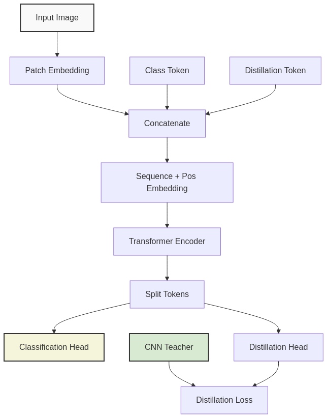
DeiT (Data-efficient image Transformers)
DeiT introduced techniques to train ViTs more efficiently on smaller datasets:
– Distillation tokens that learn from CNN teacher models
– Enhanced data augmentation strategies
– More aggressive regularization
Hierarchical Vision Transformers
Models like Swin Transformer introduced hierarchical structures similar to CNNs:
– Processing image patches at multiple resolutions,
– Using shifted windows for more efficient attention computation, and
– Creating pyramid-like feature maps suitable for dense prediction tasks.
Hybrid Approaches
Many successful models now combine CNN and Transformer components:
– ConvNeXt adds ViT design elements to CNN architectures
– Early convolutional stages before transformer layers (e.g., in CoAtNet)
– Vision Transformers with convolutional embeddings (e.g., in CvT)
Applications Beyond Classification
Vision Transformers have expanded beyond image classification to numerous vision tasks:
Object Detection and Segmentation
- DETR (DEtection TRansformer): End-to-end object detection without hand-crafted components like non-maximum suppression.
- Mask2Former: State-of-the-art segmentation using transformer decoders.
- SegFormer: Efficient transformer-based segmentation with hierarchical features.
Multi-modal Models
Transformers excel at bridging different modalities:
– CLIP (Contrastive Language-Image Pre-training): Aligns image and text representations
– DALL-E, Stable Diffusion: Text-to-image generation models that incorporate transformer components
– Flamingo: Few-shot visual and language understanding
Video Understanding
- TimeSformer: Applies self-attention across both spatial and temporal dimensions
- ViViT (Video Vision Transformer): Factorized space-time attention for video classification
Practical Considerations for Implementation
If you’re planning to implement Vision Transformers in your projects, consider these practical tips:
Data Requirements
- For small datasets (<1M images), consider using:
- Pre-trained ViT models with fine-tuning
- Hybrid models with convolutional features
- DeiT-style training with distillation
Model Selection
- ViT-Base: 12 layers, 768 hidden dimension, 12 attention heads (~86M parameters)
- ViT-Large: 24 layers, 1024 hidden dimension, 16 attention heads (~307M parameters)
- ViT-Huge: 32 layers, 1280 hidden dimension, 16 attention heads (~632M parameters)
Smaller datasets generally benefit from smaller models (Base or smaller), while larger datasets can leverage the capacity of larger models.
Training Efficiency
- Gradient checkpointing can reduce memory requirements
- Mixed precision training is essential for larger variants
- Consider sharded data parallelism for distributed training
Conclusion
ViT challenge the long-held assumption that convolutional architectures are necessary for image understanding. They demonstrate how general sequence processing architectures can, with minimal adaptation, excel at vision tasks when provided with sufficient data.
The success of ViT has broader implications for deep learning:
- Architecture unification: The boundaries between vision and language models continue to blur, enabling more powerful multi-modal systems.
- Inductive biases vs. data: With enough data, models can learn useful inductive biases rather than having them built in architecturally.
- Scalability matters: Transformer architectures are particularly amenable to scaling laws, with performance improving predictably with model size and data.
As research continues, we can expect further refinements that combine the best aspects of convolutional and transformer approaches, ultimately leading to more flexible, efficient, and powerful vision models.
Whether you’re implementing these models in production or researching new variants, understanding the fundamentals of Vision Transformers is now essential knowledge for anyone working in computer vision and deep learning.