Self-Attention and Beyond
An in-depth exploration of the mechanism that powers modern language models
1. Introduction: The Revolution of Self-Attention
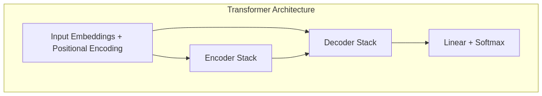
The Transformer architecture, introduced in the landmark 2017 paper “Attention Is All You Need”, has fundamentally reshaped machine learning. At its core lies the self-attention mechanism—often described as the “secret sauce” behind today’s most powerful AI models.
The concept of attention in machine translation was first introduced in the paper: “Neural Machine Translation by Jointly Learning to Align and Translate” by Dzmitry Bahdanau, Kyunghyun Cho, and Yoshua Bengio in 2014 (arXiv:1409.0473). Their paper:
- Introduced the attention mechanism in the context of sequence-to-sequence models for machine translation.
- Allowed the model to dynamically focus on different parts of the input sentence while generating each word of the output sentence.
- Overcame the limitations of fixed-length context vectors in earlier encoder-decoder architectures.
Lets compare the architectures to understand this better:
- Recurrent Neural Networks (RNNs) process tokens sequentially, creating (training) bottlenecks and struggling with long-range dependencies.
- Convolutional Neural Networks (CNNs) use fixed-size kernels, limiting their ability to capture variable-length relationships.
- Self-Attention enables direct communication between any tokens, regardless of their distance from each other.
This flexible mechanism efficiently captures both local and global dependencies while enabling massively parallel computation.

2. The Query, Key, Value Mechanism Explained
Self-attention’s elegant design revolves around three learned projections for each token:
- Query (Q): “What information am I looking for?”
Each token creates a query vector representing the type of information it needs. - Key (K): “What information do I contain?”
Each token also broadcasts a key vector advertising what information it offers. - Value (V): “What actual content do I provide?”
The value vector contains the substantive information that gets passed if the token is attended to.
In case its unclear, these vectors are from weight matrices. These weights are what the network learns during training. Don’t forget that tokens are also vectors in embedding space and will generate unique vectors upon interacting with weights. And that is why I called Q/K/V as projections.
The attention mechanism from a token’s perspective:
- For each token, compute its query vector,
- Compare this query against every token’s key vector using dot product,
- Scale the dot products and apply softmax to obtain attention weights, and
- Create the output by taking a weighted sum of the value vectors.
Mathematically:
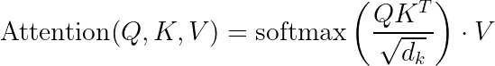
Where  is the dimension of the key vectors, and the division by
  prevents numerical instability. (I will expand on this later in the article.)
Side Note: The T is for Transpose. Imagine Q and K as arrays. Transpose of K just makes more sense to show the DOT product here and hence has become the convention.

To get a feel for it: Imagine a crowded room where each person (token) has:
– A set of questions they want answered (query),
– Topics they’re knowledgeable about (key), and
– The actual information they possess (value).
People pay more ‘attention’ to others whose expertise (keys) matches their questions (queries), and the information exchanged (values) forms their new understanding. And that is what the network learns during training!
Pro Tip: Now read through this section again and it might just make sense!
3. Self-Attention as a Dynamic Graph
Another illuminating perspective is to view self-attention as creating a dynamic, weighted graph:
- Nodes: Each token is a node in the graph
- Edges: Attention weights form directed edges between nodes
- Edge weights: The strength of connection, determined by query-key compatibility
Unlike traditional graph neural networks with fixed connectivity, self-attention creates a fully connected graph where edge weights are:
1. Learned during training
2. Computed dynamically based on input content
3. Different for every input sequence
This adaptability makes self-attention exceptionally powerful for modeling complex relationships. The attention graph essentially rewires itself for each new input, focusing on the connections most relevant to the current context.
4. Positional Information: Solving the Ordering
A critical limitation of pure self-attention is that it’s inherently permutation-invariant i.e., it treats tokens as an unordered set. This is problematic for most languages (like English), where word order carries crucial meaning.
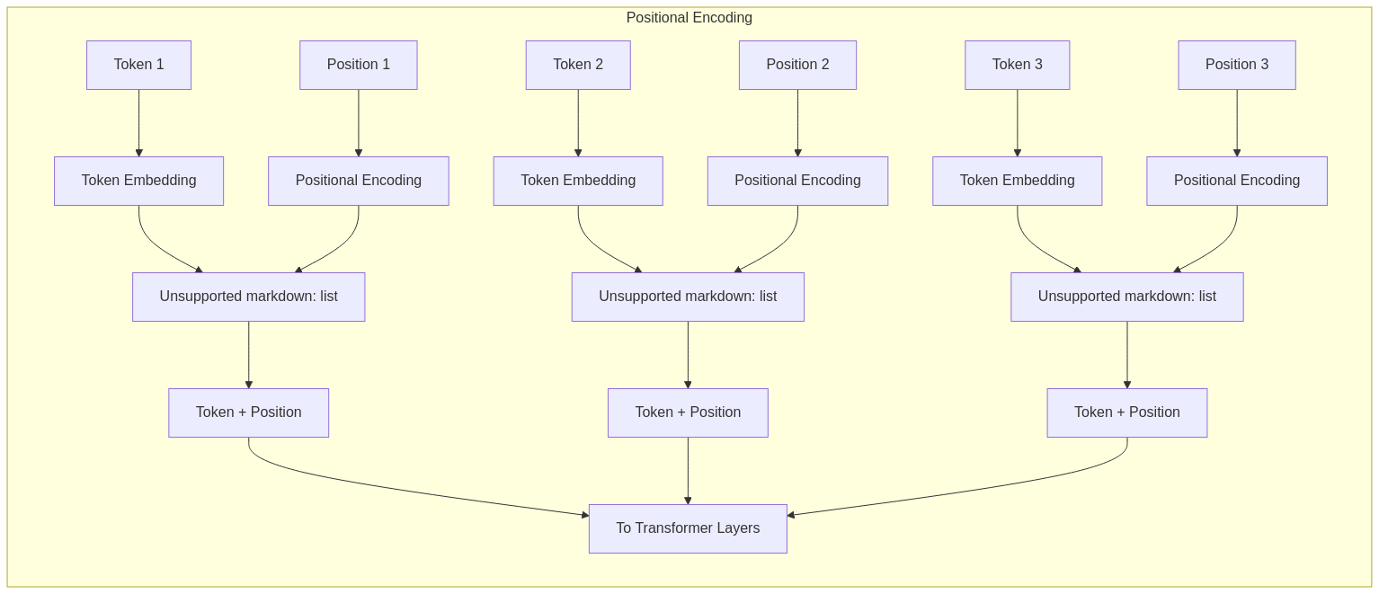
Transformers address this through positional encodings that inject “location information” into each token embedding:
Types of Positional Encodings:
1. Sinusoidal (Original Transformer): Fixed patterns of sine and cosine functions at different frequencies:
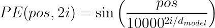

These have the nice property of enabling the model to extrapolate to sequences longer than those seen during training.
2. Learned Positional Embeddings: Directly learn a unique vector for each position (used in BERT, early GPT models).
a. Relative Positional Encoding: Encode relative distances between tokens rather than absolute positions (used in more recent models like T5).
b. Rotary Position Embedding (RoPE): Encodes position by rotating vector representations in a way that preserves their inner products (used in models like GPT-NeoX and LLaMA).
The positional information is typically added to the token embeddings before they enter the attention mechanism, enabling the model to consider both content and position simultaneously.
Comparing Positional Encoding Methods
| Method | Advantages | Disadvantages | Used in |
|---|---|---|---|
| Sinusoidal | Extrapolates to unseen sequence lengths | Fixed, not learned | Original Transformer |
| Learned | Adapts to dataset | Limited to training length | BERT, Early GPT |
| Relative | Better captures relative distances | More complex | T5, Transformer-XL |
| RoPE | Efficiently encodes in rotational space | Mathematical complexity | GPT-NeoX, LLaMA |
5. Masking: Controlling Information Flow
Transformers use different masking strategies depending on their architecture and purpose:
Padding Masks
Sequences in a batch often have different lengths and are padded to a uniform length. Padding masks prevent the model from attending to these artificial padding tokens:
Padding mask: [0, 0, 0, 0, 0, 1, 1, 1] # 0 for real tokens, 1 for padding
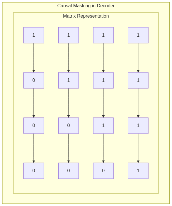
Causal (Autoregressive) Masks
In autoregressive generation (like in GPT), each token should only see previous tokens to avoid “cheating.” Causal masks implement this constraint:
For position i=3:
Causal mask: [0, 0, 0, 1, 1, 1, 1, 1]  # 0 for positions ≤ i, 1 for positions > i
Visually, a causal mask is a lower triangular matrix that zeros out attention to future positions.
Encoder vs. Decoder Attention
- Encoder Self-Attention: Bidirectional — each token attends to all tokens (with padding masks only)
- Decoder Self-Attention: Unidirectional — each token attends only to previous tokens (causal masking)
- Cross-Attention: Decoder tokens attend to all encoder tokens (only padding masks)
The masking architecture above creates the foundation for different model types:
– Encoder-only (like BERT): Bidirectional understanding
– Decoder-only (like GPT): Unidirectional generation
– Encoder-decoder (like T5): Understanding followed by generation
6. Scaling Attention and Numerical Stability
The Crucial Scaling Factor
You may be wondering about √d_k in the attention formula. Its not just a mathematical nicety.
Attention(Q, K, V) = softmax(QK^T / √d_k) × V
Without this scaling:
1. As dimensionality increases, the variance of dot products grows.
2. Large dot products push the softmax function into regions of extremely small gradients.
3. This leads to vanishing gradients and training difficulties.
The √d_k scaling factor normalizes the variance, keeping gradients in a reasonable range and enabling effective learning.
Additional Stability Techniques
Modern implementations often include:
- Attention dropout: Randomly zero out attention weights during training
- Bias terms: Adding learnable biases to Q, K, V projections
- Precision adjustments: Using mixed precision or accumulating in higher precision for attention computations
These seemingly minor details can significantly impact model performance and trainability, especially at scale.
7. Multi-Head Attention: Parallel Attention Pathways
Rather than using a single attention mechanism, Transformers employ multi-head attention, which:
- Projects the input into multiple sets of queries, keys, and values
- Computes attention independently in each “head”
- Concatenates the results and projects back to the original dimension


This parallel processing offers several advantages:
- Diverse Feature Capture: Each head can specialize in different relationship types
- Attention Redundancy: Multiple pathways provide resilience against attention failures
- Joint Representation: The combination of heads creates a richer representation than any single attention pattern
Empirical studies have revealed fascinating specializations among attention heads—some focus on syntactic relationships, others on semantic connections, coreference, or even specific linguistic phenomena.
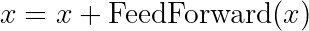
Feed-Forward Networks: Token-Wise Transformation
Following multi-head attention, each token independently passes through a position-wise feed-forward network (FFN):

This two-layer MLP with a ReLU activation:
1. Projects to a higher dimension (typically 4× the model dimension)
2. Applies non-linearity
3. Projects back to the original dimension
The FFN serves as the model’s “reasoning” component, enhancing representational capacity beyond what attention alone can achieve. Recent research suggests these FFNs may function as key-value memory stores that learn to associate patterns with appropriate outputs.
8. Residual Connections: The Gradient Superhighway
Despite their power, deep Transformer networks would be extremely difficult to train without residual connections. Also known as “skip connections”, these simply add the input of a sublayer to its output:

This elegant addition provides several crucial benefits:
- Gradient Flow: Creates direct pathways for gradients to flow backward, combating vanishing gradients.
- Information Preservation: Allows the network to retain original features while learning new ones.
- Optimization Landscape: Smooths the loss landscape, making optimization more stable.
In practice, every major component in a Transformer layer has a residual connection:

These connections effectively create an ensemble of networks of different depths, letting the model flexibly determine which transformations are necessary for each input.
9. Layer Normalization: Stabilizing the Signal
Layer Normalization (LayerNorm) normalizes the activations across the feature dimension, independently for each token:
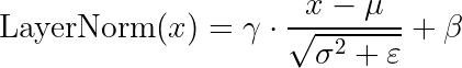
Where: –  and
and  are the mean and variance computed across the feature dimension –
  and
and  are learnable scale and shift parameters –
  is a small constant for numerical stability
LayerNorm serves several important functions:
- Training Stability: Prevents internal covariate shift
- Depth Scaling: Enables training of deeper models
- Batch Independence: Unlike BatchNorm, works well for variable-length sequences and small batches
Pre-Norm vs. Post-Norm Architecture
There are two main approaches to applying normalization:
- Post-Norm (Original Transformer): Apply LayerNorm after the residual connection
x = LayerNorm(x + Sublayer(x))
- Pre-Norm (Many modern variants): Apply LayerNorm before the sublayer
x = x + Sublayer(LayerNorm(x))
Pre-norm designs often train more stably, especially in very deep networks, while post-norm can sometimes achieve better final performance. The choice between them represents a classic stability-vs-performance tradeoff.
10. Regularization Techniques for Transformer Training
Transformers employ several regularization strategies to prevent overfitting and improve generalization:
Dropout Variants
- Attention Dropout: Randomly zeros out attention weights
- Embedding Dropout: Zeros out entire token embeddings
- Layer Dropout: Skips entire layers during training
- Hidden State Dropout: Applied after attention and FFN components
Modern Transformers often use a schedule of increasing dropout rates for larger models or longer training runs.
Weight Sharing
Some Transformer variants share parameters to improve regularization:
– Tied Embeddings: Input and output embeddings share weights.
– Shared Layer Parameters: Some models (like ALBERT) share parameters across layers.
– Universal Transformers: Recurrently apply the same Transformer layer.
Data Augmentation
Task-specific augmentation techniques include:
– Masking (like in BERT)
– Token Deletion/Insertion – Sequence Shuffling (for tasks where order isn’t critical)
– Back-Translation (for translation tasks)
The combination of these regularization strategies is crucial for training high-performing Transformer models, especially when data is limited.
11. Transformer Computation: The Complete Flow
Let’s trace the complete flow of information through a standard Transformer layer:
- Input Preparation:
- Token embeddings + positional encodings
- Apply appropriate masking patterns
- Self-Attention Block:
- Layer normalization (pre-norm variants)
- Project to queries, keys, and values across multiple heads
- Compute scaled dot-product attention:

- Concatenate heads and project
- Apply dropout
- Add residual connection
- Layer normalization (post-norm variants)
- Feed-Forward Block:
- Layer normalization (pre-norm variants)
- Expand dimension:

- Apply ReLU (or GELU in more recent models)
- Project back:

- Apply dropout
- Add residual connection
- Layer normalization (post-norm variants)
- Output Processing (final layer only):
- Task-specific heads (classification, token prediction, etc.)
This architecture repeats for N layers (anywhere from 6-12 in early models to 96+ in recent large models), with communication between layers entirely through the standard block outputs.
12. Recent Advances and Future Directions
The Transformer architecture continues to evolve rapidly:
Efficiency Innovations
- Sparse Attention: Longformer, BigBird, and Reformer use sparse attention patterns to reduce the O(n²) complexity
- Linear Attention: Performers, Linear Transformers replace softmax attention with kernel methods for O(n) complexity
- State Space Models: Mamba and similar approaches combine advantages of RNNs and Transformers
- Flash Attention: Algorithmic improvements for faster attention computation
Architectural Refinements
- Mixture of Experts: Switch Transformer, GShard add conditional computation
- Gated Mechanisms: GLU, GQA, and MQA variations enhance representational capacity
- Memory Augmentation: Extending context through external memory or retrieval
Scaling Laws and Emergent Abilities
Recent research has revealed intriguing scaling properties:
– Performance improvements follow power laws with model size.
– New capabilities emerge unpredictably at certain scale thresholds.
– Instruction tuning and RLHF unlock human-aligned behaviors.
Looking forward, key research directions include:
– Extending context length beyond current limitations.
– Enhancing reasoning capabilities through architectural innovations.
– Reducing computational requirements for both training and inference.
– Improving alignment with human values and intentions.
13. Conclusion: The Transformer Legacy
The Transformer architecture represents one of the most significant innovations in modern machine learning. Its attention-based design has:
- Revolutionized natural language processing by enabling unprecedented language understanding and generation
- Transcended domains to excel in vision, audio, biological sequences, and multimodal tasks
- Scaled efficiently from small specialized models to today’s frontier large language models
- Inspired new research directions across machine learning and artificial intelligence
While future architectures may eventually supplant aspects of the Transformer design, its core insights, particularly the self-attention mechanism, have fundamentally changed how we approach sequence modeling and will continue to influence AI research for years to come.
The elegance of the Transformer lies in its balance of simplicity and expressiveness: a handful of carefully designed components that, when combined, create systems capable of remarkable feats of language understanding, reasoning, and generation. As researchers continue to refine and extend this architecture, we can expect even more impressive capabilities to emerge.
Further Reading & References
- Vaswani et al. (2017): “Attention Is All You Need” – The original Transformer paper
- He et al. (2015): “Deep Residual Learning for Image Recognition” – Introduces residual connections
- Ba et al. (2016): “Layer Normalization” – Introduces LayerNorm
- Devlin et al. (2018): “BERT: Pre-training of Deep Bidirectional Transformers for Language Understanding” – Encoder-only Transformer
- Radford et al. (2018, 2019, 2020): The GPT series papers – Decoder-only Transformers
- Brown et al. (2020): “Language Models are Few-Shot Learners” – GPT-3 and scaling laws
- Dosovitskiy et al. (2020): “An Image is Worth 16×16 Words: Transformers for Image Recognition at Scale” – Vision Transformer (ViT)
- Hoffmann et al. (2022): “Training Compute-Optimal Large Language Models” – Chinchilla scaling laws
- Touvron et al. (2023): “LLaMA: Open and Efficient Foundation Language Models” – Recent open-source LLM architecture
The remarkable adaptability of Transformer architectures means that this story continues to unfold. What started as a novel approach to machine translation has evolved into a foundational technology powering the most capable AI systems we’ve ever built—a testament to the power of attention-based mechanisms for modeling complex data.
[…] would help if you have an understanding of the Transformer architecture before exploring this […]