Mamba: Linear-Time Sequence Modeling Beyond Transformers

Introduction: The Search for Efficient Sequence Models

Transformers have ruled the sequence modeling roost since 2017, their attention mechanism a powerful lens for capturing relationships across data. But power demands a price. As we shove ever-longer sequences—thousands, potentially millions of tokens—down their throats, the $O(n^2)$ complexity bites. Hard. It’s not just expensive; it’s a fundamental computational wall, a practical barrier limiting our ambitions. The search for alternatives isn’t mere academic curiosity; it’s driven by the necessity of finding a path through that wall. Enter Mamba, an architecture born from this need, promising linear-time scaling without crippling performance trade-offs.

1. The Landscape of Sequence Modeling: Strengths and Limitations

Before diving into Mamba, let’s survey the terrain and understand the trade-offs inherent in existing approaches. Each has its virtues, each its Achilles’ heel.

1.1 Transformers: Power at a Cost

Transformers changed the game with attention, allowing models to weigh the importance of tokens regardless of distance. A genuine breakthrough.
But the party doesn’t last forever. The limitations are baked into the architecture:
1. Quadratic scaling: The $O(n^2)$ compute and memory cost with sequence length isn’t just a footnote; it’s a crippling constraint for truly long contexts.
2. Context window constraints: Practical limits emerge quickly, bottlenecking applications that need to ingest massive amounts of information.
3. Computational inefficiency: Beyond a certain length, Transformers become prohibitively slow and expensive to train and run. The physics of $n^2$ is unforgiving.

1.2 Convolutions: Local but Limited

Convolutional Neural Networks (CNNs) are masters of local patterns, using sliding kernels to efficiently extract spatial or sequential features.
For sequence modeling, however, they are fundamentally short-sighted:
- Fixed receptive fields: Capturing long-range dependencies requires stacking many layers – a brute-force approach that often yields diminishing returns and architectural bloat.
- Lack of dynamic context processing: They lack the fluid, context-dependent weighting that attention provides so naturally.
- Inefficiency at scale: Increasing the effective receptive field significantly can become computationally taxing in its own right.

1.3 The Recurrent Approach: RNNs and Their Evolution

Recurrent Neural Networks (RNNs) process sequences element by element, carrying a hidden state meant to summarize the past. Conceptually elegant.
In practice, classic RNNs carried significant historical baggage:
1. Sequential processing: Inherently difficult to parallelize efficiently on modern hardware. A major bottleneck.
2. Vanishing/exploding gradients: The bane of training deep recurrent models, making it hard to capture truly long-term dependencies.
3. Limited capacity: Simple RNNs often struggled to model the intricate dependencies present in complex sequences like natural language.
LSTM and GRU architectures introduced gating mechanisms, offering clever patches to the gradient problems. But they couldn’t fully escape the sequential processing limitation.

1.4 Linear RNNs: Streamlining Recurrence

A linear RNN simplifies the recurrence, removing internal nonlinearities: $x_{k} = A \, x_{k-1} + B \, u_k, \quad y_k = C \, x_k.$ where $x_k$ is the hidden state, $u_k$ the input, $y_k$ the output, and $A,B,C$ are learned matrices.
This linearity offers potential advantages:
- Parallelized computation: The linear recurrence can often be computed efficiently using scan operations.
- Stable gradient flow: Easier to manage gradients with appropriate initialization.
- Efficient scaling: Potentially better scaling for long sequences.

However, the elegance came at the cost of expressivity. Standard linear RNNs proved too blunt an instrument for complex tasks due to:

Static processing: The same $A, B, C$ matrices applied regardless of the input context.
Inability to selectively filter: No mechanism to prioritize or ignore information dynamically.
Fixed dynamics: The model’s behavior couldn’t adapt to the nuances of the input sequence.

1.5 State Space Models (SSMs): Continuous Recurrence

State Space Models provided a fresh perspective, often framing the recurrence in continuous time: $\frac{d}{dt} x(t) = A\, x(t) + B \, u(t), \quad y(t) = C \, x(t).$
Breakthroughs like S4 (Structured State-Space for Sequence Modeling) showed that by carefully parameterizing these models (particularly the $A$ matrix) and using sophisticated discretization and computation techniques, SSMs could effectively model long-range dependencies, challenging Transformers in specific domains.
Despite these advances, traditional SSMs still suffered from the stiffness of time-invariant parameters ( $A, B, C$ are fixed). They lacked the dynamic adaptability needed to truly handle the complexity and variability of data like natural language.

2. Mamba: Adaptive State Spaces for Efficient Sequence Modeling

Mamba doesn’t just tweak the SSM formula; it injects adaptability at its core. The breakthrough? Making the state transition itself data-dependent. A selective state space model. This seemingly simple change addresses the core limitation of prior SSMs and linear RNNs. The name “Mamba” itself is a nod to its mathematical lineage ( $\text{Ma}$ trix $\text{A}$ + $\text{m}$ gating) and its intended speed – processing sequences rapidly, like its namesake.

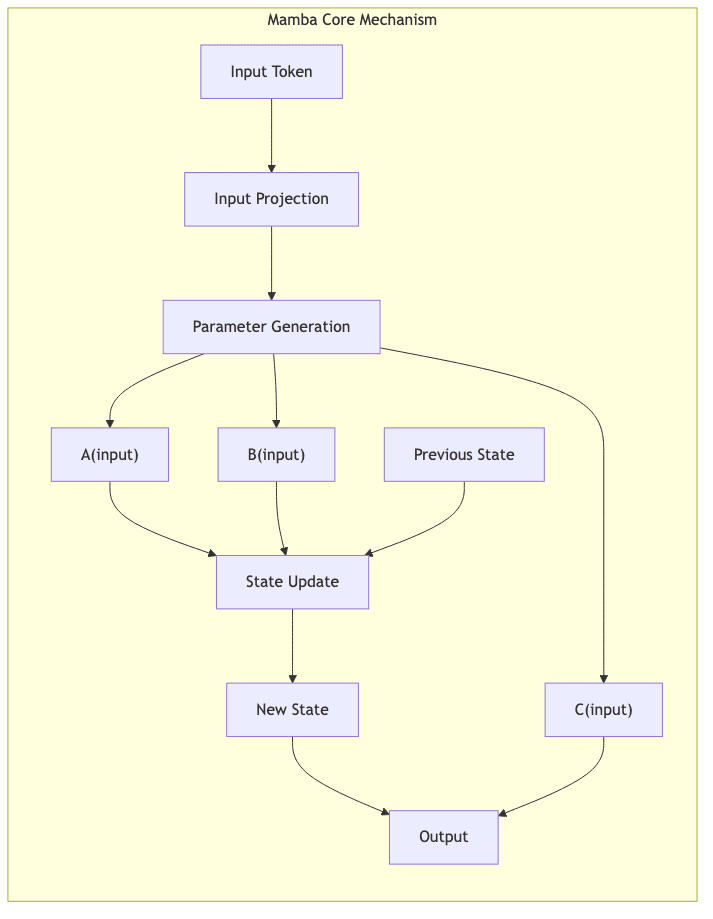
2.1 The Core Innovation: Input-Dependent Dynamics

Mamba’s key insight is to replace the static $A, B, C$ parameters of traditional SSMs with parameters that are functions of the current input $u_k$ : $\begin{aligned} x_{k} &= A_k \, x_{k-1} + B_k \, u_k,\\ y_{k} &= C_k \, x_{k}, \end{aligned}$

Where $A_k$ , $B_k$ , and $C_k$ are generated dynamically based on $u_k$ . This allows the model to:

Selectively manage information flow: The model learns to decide, based on the input, what information from its past state ( $x_{k-1}$ ) is relevant and should be kept, and what can be discarded or compressed.
Perform input-dependent processing: The way the current input $u_k$ influences the state update depends on the input itself. It’s conceptually similar to attention’s goal of dynamic weighting, but achieved through a linear-time recurrent mechanism.
Exhibit adaptive recurrent dynamics: The fundamental behavior of the recurrence changes on the fly, allowing it to adapt to different patterns and contexts within the sequence. It breaks the tyranny of fixed parameters.

2.2 Technical Advantages of Mamba

Mamba’s design translates into several significant advantages:

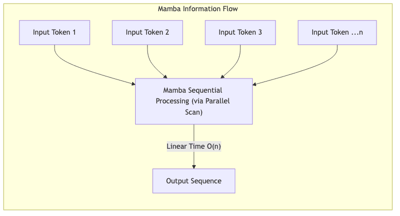
Linear-time processing: This is the headline. Both training and inference scale linearly, $O(n)$ , with sequence length. This fundamentally breaks the $O(n^2)$ bottleneck of vanilla Transformers.
Efficient long-range modeling: The recurrent nature allows information to propagate across arbitrary distances without the quadratic memory and compute cost of full attention.
Selective state updating: This is the how. Unlike traditional SSMs, Mamba can dynamically filter and prioritize information based on input relevance, giving it greater expressive power.
Hardware efficiency: The architecture is explicitly designed with modern GPU/TPU capabilities in mind, leveraging optimized scan operations for practical speed, especially crucial for inference. This is the practical payoff.

2.3 Complexity Comparison: Mamba vs. Transformers

Complexity Metric	Mamba	Vanilla Transformer	Efficient Transformer Variants
Inference Time	$O(n)$	$O(n^2)$	$O(n \log n)$ or $O(n)$
Training Time	$O(n)$	$O(n^2)$	$O(n \log n)$ or $O(n)$
Memory Usage	$O(n)$	$O(n^2)$	$O(n \log n)$ or $O(n)$
Context Length Scaling	Linear	Quadratic	Sub-quadratic

The table starkly illustrates Mamba’s advantage. While various “efficient Transformers” attempt to mitigate the quadratic cost, Mamba achieves true linear scaling in time and memory. This is precisely why it’s generating excitement for applications demanding context windows far beyond what standard Transformers can handle (10k+ tokens and potentially much more).

3. The Mathematical Framework Behind Mamba

3.1 From Linear RNNs to State Space Models

Understanding Mamba requires appreciating the lineage from discrete linear RNNs to their continuous SSM counterparts, which S4 successfully leveraged:

Discrete Linear RNN: Simple, but limited. $\begin{aligned} x_{k} &= A\,x_{k-1} + B\,u_{k}, \\ y_{k} &= C\,x_k. \end{aligned}$
Continuous State Space Model: Theoretically powerful for long dependencies. $\frac{d}{dt}x(t) = A\,x(t) + B\,u(t), \quad y(t) = C\,x(t).$

SSMs, particularly structured variants like S4, showed how careful discretization and specialized algorithms (like representing $A$ via HiPPO matrices) could bridge this gap and capture long-range dependencies effectively. However, they remained bound by time-invariant $A, B, C$ .

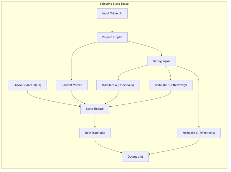
3.2 Selective State Space Mechanism

Mamba breaks this time-invariance. The core mechanism makes the effective $A_k$ , $B_k$ , $C_k$ parameters dynamic functions of the input $u_k$ :

$x_{k} = A(u_k) \, x_{k-1} + B(u_k) \, u_k, \quad y_k = C(u_k)\,x_k,$ (Note: This is a conceptual representation; the actual implementation involves gating mechanisms and projections)

This selection is typically achieved through:

Project & Gate: The input token $u_k$ is projected, and parts of this projection are used to compute gating signals (e.g., via sigmoid or SiLU activations).
Parameter Generation: These gating signals dynamically modulate the base SSM parameters or influence how the input interacts with the state, effectively creating input-dependent $A_k, B_k, C_k$ .
Selective Filtering: By controlling these dynamic parameters, the model learns to selectively propagate or forget information in its hidden state $x_k$ . It gains the ability to focus.

3.3 Fast Computation Through Hardware-Aware Design

The theoretical elegance of linear-time recurrence needs essential engineering to become practical speed on silicon. Mamba achieves this through:

Scan-based Implementation: Leveraging parallel prefix sum (scan) algorithms to compute the recurrent updates in parallel, avoiding sequential loops.
Specialized CUDA Kernels: Custom, optimized implementations for modern GPUs that fuse operations and manage memory efficiently.
Hardware-Aware Operations: Designing the computations (like the discretization of A) to map well onto hardware primitives.

These are not just optimizations; they are the bridge from mathematical theory to practical, high-throughput computation.

4. Mamba Architecture: Building Blocks and Implementation

4.1 Core Components of a Mamba Block

Like Transformers, Mamba models are typically built by stacking blocks. A standard Mamba block often includes:

Token Embedding/Input Projection: Mapping input tokens/vectors to the model’s working dimension.
Convolutional Gating (Optional but common): A small 1D convolution often applied before the SSM layer to incorporate local context.
Selective SSM Layer: The core Mamba mechanism with dynamic parameter generation and state update.
Activation/Normalization: Standard components like LayerNorm and activation functions (e.g., SiLU).
Feed-Forward Expansion (Optional): Sometimes included for additional processing capacity.
Residual Connections: Essential for deep architectures, allowing gradients to flow easily.

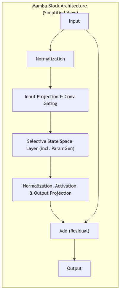
(Note: The specific arrangement and inclusion of components like Feed-Forward layers can vary between Mamba implementations. The diagram above presents a simplified residual block structure incorporating the core SSM.)

4.2 Parameter Generation and Selection Mechanism

The “selection” happens implicitly through how the input $u_k$ dynamically modifies the $A, B, C$ parameters used in the state update:

Computing Selection Signals: Input projections are passed through linear layers and activations (like SiLU) to create gating signals.
Modulating State Updates: These gates control how the discretized $A$ matrix affects the state decay and how the input $B_k u_k$ updates the state.
Controlling Information Flow: This allows the model to learn context-dependent filtering – preserving relevant history, forgetting irrelevant details, analogous to attention’s weighting but implemented via efficient recurrence.

4.3 Architectural Design Choices

Building effective Mamba models involves several tuning parameters and design choices:

State Expansion Ratio ( $N$ ): The dimension of the latent state $x_k$ . A larger $N$ increases capacity but also computational cost.
Model Dimension ( $D$ ): The main hidden dimension of the model.
Convolution Kernel Size ( $K$ ): Size of the optional 1D convolution.
Discretization Method: Techniques like Zero-Order Hold (ZOH) or Bilinear Transform (used in S4) to convert continuous $A, B$ to discrete $A_k, B_k$ .
Initialization Strategy: Careful initialization (e.g., linking $A$ initialization to the HiPPO framework from S4) is crucial for stability.

These are trade-offs architects must navigate to balance performance, efficiency, and stability.

5. Implementation Details: From Theory to Practice

5.1 Pseudocode for a Mamba Block

The following pseudocode illustrates the logic of a Mamba block. Crucially, real implementations replace the sequential loop with highly optimized parallel scan operations.

import torch
import torch.nn as nn

class MambaBlock(nn.Module):
    def __init__(self, d_model, d_state, d_conv=4, expand_factor=2):
        super().__init__()
        # Dimensions
        self.d_model = d_model
        self.d_state = d_state # N
        self.d_conv = d_conv
        self.d_inner = int(expand_factor * d_model) # D * E
        
        # Projections for input x and gating z
        self.in_proj = nn.Linear(d_model, 2 * self.d_inner, bias=False) 
        self.out_proj = nn.Linear(self.d_inner, d_model, bias=False)
        
        # Convolutional layer for local context
        self.conv1d = nn.Conv1d(
            in_channels=self.d_inner,
            out_channels=self.d_inner,
            kernel_size=d_conv,
            padding=d_conv - 1,
            groups=self.d_inner,
            bias=True
        )
        
        # Activation
        self.activation = nn.SiLU()

        # SSM parameters (A, B, C, Delta)
        # Projections for Delta, B, C (generate parameters based on input)
        self.x_proj = nn.Linear(self.d_inner, d_state + 2 * d_state, bias=False) # Project for delta, B, C
        
        # Learnable log of time step Delta and log of A matrix
        self.dt_rank = self.d_inner // 16 # Rank for delta projection
        self.delta_proj = nn.Linear(self.dt_rank, self.d_inner, bias=True)
        self.A_log = nn.Parameter(torch.randn(self.d_inner, d_state)) # log(A)
        
        # Learnable D matrix (skip connection)
        self.D = nn.Parameter(torch.ones(self.d_inner))

    def forward(self, x):
        # x: [batch_size, seq_len, d_model]
        batch, seq_len, _ = x.shape
        
        # Input projection: Split into x and z pathways
        xz = self.in_proj(x) # [B, L, 2 * d_inner]
        x_input, z = xz.chunk(2, dim=-1) # x_input: [B, L, d_inner], z: [B, L, d_inner]

        # Apply convolution, activation, and projection for SSM parameters
        x_conv = self.conv1d(x_input.transpose(1, 2))[:, :, :seq_len] # [B, d_inner, L]
        x_conv = self.activation(x_conv).transpose(1, 2) # [B, L, d_inner]
        
        # Project x_conv to get delta, B, C
        x_ssm = self.x_proj(x_conv) # [B, L, dt_rank + 2*d_state]
        delta, B, C = torch.split(x_ssm, [self.dt_rank, self.d_state, self.d_state], dim=-1) # delta:[B,L,rank], B:[B,L,N], C:[B,L,N]
        
        # Compute Delta_t (learnable time step)
        delta = torch.nn.functional.softplus(self.delta_proj(delta)) # [B, L, d_inner]

        # --- Core SSM Calculation (Simplified Loop - Real code uses scan) ---
        A = -torch.exp(self.A_log.float()) # [d_inner, N]
        D = self.D.float()

        # Discretize A and B using Zero-Order Hold (ZOH)
        # delta_A = exp(delta * A)
        # delta_B = (exp(delta * A) - 1) / A * B --- simplified here
        # (requires careful handling when A is near zero)
        
        h = torch.zeros(batch, self.d_inner, self.d_state, device=x.device) # Initial state [B, d_inner, N]
        ys = []

        # THIS LOOP IS FOR ILLUSTRATION ONLY - PRODUCTION USES PARALLEL SCAN
        for i in range(seq_len):
            delta_i = delta[:, i].unsqueeze(-1) # [B, d_inner, 1]
            A_i = torch.exp(delta_i * A) # [B, d_inner, N] - Discretized A
            B_i = delta_i * B[:, i] # [B, d_inner, N] - Simplified discretized B
            
            h = A_i * h + B_i * x_conv[:, i].unsqueeze(-1) # [B, d_inner, N] - State update
            y = (h * C[:, i].unsqueeze(1)).sum(dim=-1) # [B, d_inner] - Output computation
            ys.append(y)
        
        y = torch.stack(ys, dim=1) # [B, L, d_inner]
        # --- End Simplified Loop ---

        # Apply skip connection D * x_input
        y = y + x_input * D 
        
        # Apply gating z
        y = y * self.activation(z) # [B, L, d_inner]
        
        # Output projection
        output = self.out_proj(y) # [B, L, d_model]
        return output

Note: The provided pseudocode is illustrative and simplifies aspects like discretization and the scan operation for clarity. Consult official implementations for precise details.

5.2 Optimizations for Training and Inference

Achieving Mamba’s practical speed relies heavily on sophisticated engineering beyond the basic math:

Parallel Scan Algorithms: The absolute key. Re-expressing the sequential recurrence $h_t = A_t h_{t-1} + B_t u_t$ as a parallel scan allows computation in $O(L \log L)$ or even $O(L)$ work on parallel hardware, depending on the algorithm variant.
Memory-Efficient Backpropagation: Standard backpropagation through the unrolled recurrence would be memory-intensive. Checkpointing or specialized scan-based gradient computation is needed.
Fused Operations: Kernels often fuse multiple steps (e.g., discretization, state update, output calculation) to minimize GPU memory reads/writes, a common bottleneck.
Quantization-Friendly Design: Choices made in the architecture can impact how well the model performs when weights and activations are quantized to lower precision (e.g., INT8) for faster inference.

These optimizations are crucial for realizing the theoretical linear-time promise on actual hardware.

6. Applications and Performance: Where Mamba Excels

6.1 Language Modeling Performance

Early benchmarks indicate that Mamba is not just efficient, but also powerful. It achieves language modeling performance (e.g., perplexity) competitive with state-of-the-art Transformer models of similar parameter counts, while offering:

Dramatically better scaling: Performance degrades much more gracefully as sequence length increases.
Faster inference: Particularly noticeable in autoregressive generation tasks where each token depends on the previous state.
Reduced training cost: For very long sequences, the linear scaling translates to significant savings in compute time and resources.

6.2 Long-Context Applications

Mamba’s linear scaling is an enabler for applications previously choked by quadratic complexity:

Document-level understanding/summarization: Processing entire books or lengthy reports in one go.
Time-series analysis: Modeling financial, sensor, or climate data with extremely long historical dependencies.
Genomic sequence modeling: Handling DNA/RNA sequences that can be millions or billions of elements long.
Code generation and analysis: Understanding entire codebases or long development histories.

These are domains where the $O(n^2)$ cost of Transformers becomes an insurmountable barrier.

6.3 Resource Efficiency

The architectural advantages translate directly into real-world benefits during deployment:

Lower inference memory: Storing the recurrent state is typically much cheaper than storing the entire $N \times N$ attention matrix or KV cache for Transformers, especially at long lengths.
Faster decoding: Autoregressive generation requires only a single step of the recurrence per token, potentially faster than attention-based decoding.
Improved hardware utilization: The scan-based approach can be optimized to saturate modern compute units effectively.

7. Conclusion: The Future of Sequence Modeling

Mamba seems like a genuine architectural contender, tackling the Transformer’s quadratic bottleneck head-on by cleverly merging the structure of SSMs with input-dependent selectivity. The result? Linear-time scaling, opening the door to ultra-long context applications where Transformers simply choke. It achieves this through a combination of:

The efficiency of parallelizable recurrence (building on SSMs)
The power of adaptive, input-dependent dynamics (its key innovation)
The necessity of hardware-aware algorithms (making theory practical)

Mamba delivers a compelling blend of computational efficiency and modeling capability.

7.1 Current Limitations and Future Work

Despite the promise, Mamba is still nascent compared to the mature Transformer ecosystem:

Tooling and Infrastructure: Less off-the-shelf support in major libraries compared to Transformers (though this is rapidly changing).
Interpretability: Understanding why Mamba makes certain predictions is arguably harder than analyzing attention maps. Visualizing the dynamic state evolution is an open area.
Architecture Exploration: As a newer architecture, the optimal configuration and training recipes are still being actively researched.

7.2 Broader Implications

Mamba’s emergence is significant. It proves that fundamental architectural innovation beyond attention is still possible and potent. It underscores that revisiting older concepts (like recurrence) with modern mathematical tools and hardware-aware engineering can lead to breakthroughs.

As our need to process ever-larger amounts of sequential data grows—from analysing novels to decoding genomes—architectures like Mamba, designed with computational scaling as a first principle, are not just interesting; they are likely essential. The physics of computation continues to shape the frontiers of AI.

References & Further Reading

Mamba Paper: Gu, A., & Dao, T. (2023). “Mamba: Linear-Time Sequence Modeling with Selective State Spaces.” arXiv:2312.00752
S4 Paper: Gu, A., Goel, K., Ré, C. (2021). “Efficiently Modeling Long Sequences with Structured State Spaces.” ICLR 2022
Transformers: Vaswani, A., Shazeer, N., Parmar, N., Uszkoreit, J., Jones, L., Gomez, A. N., Kaiser, Ł., & Polosukhin, I. (2017). “Attention Is All You Need.” NeurIPS 2017
RNNs: Elman, J. L. (1990). “Finding structure in time.” Cognitive Science
LSTMs: Hochreiter, S., & Schmidhuber, J. (1997). “Long Short-Term Memory.” Neural Computation

Note: This article provides an overview of Mamba based on information available up to its specified date. Research in AI architectures evolves rapidly; always consult the latest publications for the most current understanding and performance benchmarks.

Posted in AI / ML, LLM Research by Rakshit Kalra

Write a comment