FlashAttention: Revolutionizing Transformer Efficiency

1. Understanding Attention in Transformers

1.1 The Standard Attention Formula

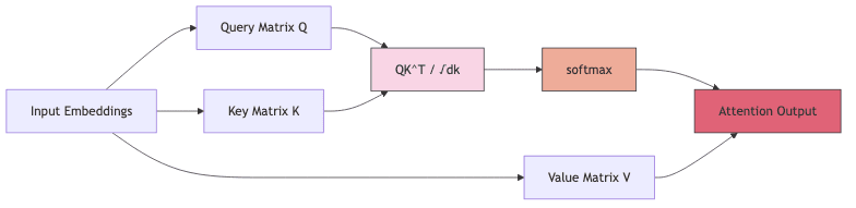
Self-attention is the magic ingredient, the mechanism letting Transformers understand context by weighing the relevance of different parts of an input sequence to each other. The core math looks deceptively simple:

$\textrm{Attention}(Q, K, V) = \textrm{softmax}\left(\frac{Q K^T}{\sqrt{d_k}}\right) V,$

Where:

$Q, K, V$ are the query, key, and value matrices, derived projections of the input embeddings. Think of them as different perspectives on the input data.
Each matrix has shape ((N, d)) for a single attention head (where $N$ is the sequence length and $d$ is the embedding dimension).
In multi-head attention (the standard practice), we split $d$ into $h$ heads, each working on a smaller dimension $d_{\textrm{head}} = d/h$ . More perspectives.
$\sqrt{d_k}$ is the scaling factor, usually $\sqrt{d_{\textrm{head}}}$ , a small but crucial detail to keep gradients from exploding during training. Stability matters.
$\textrm{softmax}$ does its usual job: applied row-wise to the $QK^T$ scores, turning them into probabilities or weights that sum to 1.

This formula allows the model, for each token, to dynamically decide which other tokens deserve its focus, creating rich, context-aware representations. It’s clever.

1.2 The Quadratic Scaling Problem

Here’s the rub. That elegance comes at a steep price, particularly as sequences get longer (and they always need to get longer):

Computational Grind: Calculating the $QK^T$ matrix requires (O(N^2 d)) operations. That $N^2$ term bites. Hard. Double the sequence length, quadruple the compute for this step.
Memory Hog: Just storing the intermediate $N \times N$ attention matrix (\text{softmax}(QK^T/\sqrt{d_k})) eats (O(N^2)) memory. For sequences of thousands or tens of thousands of tokens, this becomes astronomical.
Training Tax: Backpropagation needs intermediate values. Standard attention implementations have to stash even more data, exacerbating the memory pressure.

Modern models routinely chew on sequences in the thousands. That $N^2$ isn’t theoretical; it’s a brick wall. The attention mechanism, the very source of the Transformer’s power, became its primary scaling bottleneck. We needed a better way, not just incrementally faster, but fundamentally more efficient in terms of memory.

2. The FlashAttention Breakthrough

2.1 Beyond Approximation Methods

For a while, the community chased two main approaches to tame the quadratic beast:

Sparse Attention: Clever tricks to compute attention only for some pairs of tokens, assuming (hoping?) that most interactions aren’t critical (e.g., Sparse Transformers, BigBird).
Low-Rank Approximations: Mathematical gymnastics to approximate the attention matrix using lower-dimensional projections, essentially compressing it (e.g., Linformer, Performer).

These methods often worked, reducing complexity, but they came with trade-offs. Model quality could suffer. Hyperparameters needed finicky tuning. They felt like patches, workarounds. FlashAttention arrived with a different philosophy: don’t approximate, optimize. Compute the exact same attention, but do it without the crippling memory overhead.

2.2 The IO-Aware Approach

The core insight of FlashAttention is deceptively simple but profound: modern GPUs are often starved for data, not computational power. The real bottleneck isn’t the number of calculations (FLOPS), but the time spent shuffling data between the GPU’s fast-but-small SRAM and its large-but-slow High Bandwidth Memory (HBM or DRAM). FlashAttention is explicitly IO-aware. It restructures the computation to minimize this costly data movement:

Divide and Conquer: Break the input Q, K, V matrices into blocks small enough to fit into the GPU’s fast SRAM.
Tiling: Process these blocks (tiles) iteratively. Compute attention scores and update the output block-by-block without ever forming the full $N \times N$ attention matrix in memory.
On-Chip Accumulation: Keep the running sums and normalization factors (needed for the eventual softmax) directly in ultra-fast GPU registers or shared memory (SRAM).
Memory Hierarchy Management: Orchestrate the data flow meticulously, maximizing the use of fast on-chip memory and minimizing trips to the slower main GPU DRAM.

GPU["GPU Memory Hierarchy (The Battleground)"]

It’s the same math, the same final numbers, but achieved by respecting the physical realities of the hardware. By minimizing memory reads/writes, FlashAttention attacks the true bottleneck.

3. The Mathematics Behind FlashAttention

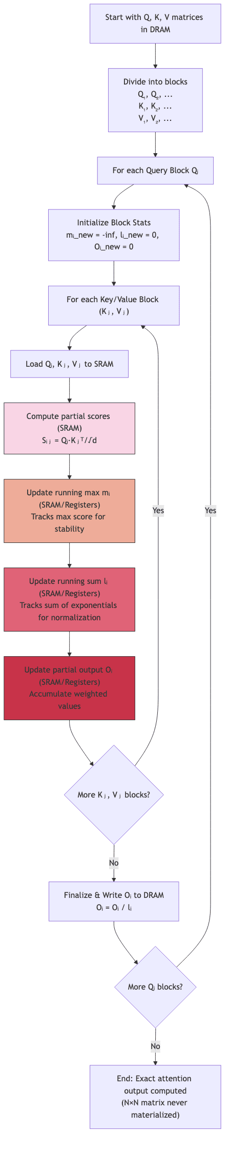
3.1 Blockwise Softmax: The Core Innovation

How can you compute softmax without seeing the whole input vector? The key is realizing that softmax can be computed block-by-block using the log-sum-exp trick for numerical stability and some careful bookkeeping. Imagine dividing the N-length sequence into blocks of size $B$ . The algorithm proceeds roughly like this:

Iterate through blocks of queries $Q_i$ .
For each query block $Q_i$ , iterate through blocks of keys and values ((K_j, V_j)).
Compute the attention scores for this block pair: $S_{ij} = Q_i K_j^T / \sqrt{d_k}$ . This small $B \times B$ matrix does fit in SRAM.
Crucially, update running statistics for each query row i: the maximum score seen so far ( $m_i$ ) and the sum of exponentiated scores ( $l_i$ ). These are needed for the final normalization.
Update the output block $O_i$ incrementally using the current block’s scores and values $V_j$ , rescaling based on the running statistics.

The specific update rules maintain numerical stability while ensuring the final output is identical to standard softmax:

$m_i^{\textrm{new}} = \max(m_i^{\textrm{old}}, \max_{\textrm{cols}}(S_{ij})) \quad \textrm{// Track max for numerical stability}$

$l_i^{\textrm{new}} = l_i^{\textrm{old}} \cdot e^{m_i^{\textrm{old}} - m_i^{\textrm{new}}} + \sum_{\textrm{cols}} e^{S_{ij} - m_i^{\textrm{new}}} \quad \textrm{// Update sum of exps, rescaling previous}$

$O_i^{\textrm{new}} = O_i^{\textrm{old}} \cdot e^{m_i^{\textrm{old}} - m_i^{\textrm{new}}} + \sum_{\textrm{cols}} \left(e^{S_{ij} - m_i^{\textrm{new}}} \cdot V_j\right) \quad \textrm{// Update output, rescaling previous}$

The beauty is that the full $N \times N$ matrix $S$ or the final softmax probability matrix $P$ never needs to be stored in GPU memory. It lives ephemerally, block by block, within the fast SRAM.

3.2 Memory Efficiency Analysis

The difference in memory footprint is dramatic:

Standard Attention: Needs (O(N^2)) memory just for the attention matrix, plus (O(Nd)) for Q, K, V, and outputs. Backpropagation often requires saving the (O(N^2)) matrix, making things even worse.
FlashAttention: Requires only (O(Nd)) memory for Q, K, V, and outputs. The only quadratic term is within the tiny block computation, (O(B^2)), which is negligible as $B$ is small (e.g., 64 or 128) and happens in SRAM.

For sequences stretching into the many thousands ( $N = 10,000+$ ), this is more than algo optimization; it’s the difference between running a model and hitting an out-of-memory (OOM) wall. The memory savings, especially during training (including the backward pass), are enormous.

4. FlashAttention 2: Further Innovations

Never content, the researchers behind FlashAttention quickly followed up with FlashAttention 2, squeezing out even more performance by refining the initial concept:

Better Parallelism: Re-engineered the parallel reduction operations for the blockwise softmax, improving GPU core utilization.
Smarter Work Partitioning: More carefully balanced the workload across different thread blocks and warps on the GPU, reducing idle time.
Kernel Fusion: Fused more operations together, further minimizing memory transfers.
Hardware Awareness: Tuned implementations specifically for the nuances of different GPU generations (like NVIDIA’s A100 vs. H100).

These weren’t fundamental algorithmic changes, but rather relentless engineering optimization, building on the IO-aware foundation. The result? Up to another 30% speed boost over the already impressive original FlashAttention, while preserving the crucial memory efficiency. The backward pass received similar treatment, ensuring gradients could be computed just as efficiently.

5. Performance Benchmarks: Seeing is Believing

Talk is cheap. The benchmarks show the real story:

Configuration	Standard Attention (PyTorch)	FlashAttention 2	Speedup	Memory Footprint	Can it Run?
Batch=4, Seq=1024, d=1024	1.0× (baseline)	~2.0-2.5× faster	~2.0-2.5×	Dramatically Lower	Yes
Batch=8, Seq=2048, d=1536	1.0× (baseline)	~2.3-3.0× faster	~2.3-3.0×	Dramatically Lower	Yes
Batch=8, Seq=8192, d=2048	OOM (Out of Memory)	Works (~ms per step)	∞	Manageable	Only with Flash

(Note: Specific numbers vary based on GPU, precision, etc. The trend is consistent.) The advantages amplify dramatically with longer sequences. Where standard attention simply crashes due to memory limits, FlashAttention sails through. This enables training configurations and context lengths that were previously impossible on given hardware. And crucially, this speed comes without approximation. It’s the same mathematical result, just computed far more intelligently.

6. The Ecosystem of Fused Operations

FlashAttention is a star player, but it performs best as part of a team. Its memory-saving philosophy complements other “fused” operations common in modern Transformers, where multiple distinct mathematical steps are combined into a single GPU kernel to minimize memory round-trips.

6.1 Fused LayerNorm

Layer Normalization is ubiquitous: $\textrm{LayerNorm}(x) = \frac{x - \mu}{\sqrt{\sigma^2 + \epsilon}} \cdot \gamma + \beta$ Calculating mean ( $\mu$ ), variance ( $\sigma^2$ ), normalizing, and applying scale ( $\gamma$ ) and bias ( $\beta$ ) normally involves several passes over the data. Fusing them into one kernel saves significant memory bandwidth.

6.2 Fused Activation Functions

Activations like GeLU or SwiGLU are common: $\textrm{SwiGLU}(x, W_1, W_2, b_1, b_2) = \left(\sigma(x W_1 + b_1) \odot (x W_2 + b_2)\right)$ Fusing the linear projections, the sigmoid ( $\sigma$ ), and the element-wise multiplication ( $\odot$ ) reduces intermediate memory usage.

6.3 Optimized Positional Encodings

Rotary Positional Embeddings (RoPE) inject position information by rotating pairs of query/key dimensions: $\begin{pmatrix} q'_{\textrm{even}} \\ q'_{\textrm{odd}} \end{pmatrix} = \begin{pmatrix} q_{\textrm{even}} \cos(\theta_m) - q_{\textrm{odd}} \sin(\theta_m) \\ q_{\textrm{even}} \sin(\theta_m) + q_{\textrm{odd}} \cos(\theta_m) \end{pmatrix}$ Applying these rotations within the attention kernel, rather than as a separate step requiring another memory read/write, adds to the overall efficiency. Combining FlashAttention with fused LayerNorm, activations, and positional encodings makes the entire Transformer block vastly more memory-efficient, paving the way for larger models and longer contexts on existing hardware.

7. Flash Decoding: Transforming Inference

The benefits aren’t limited to training. The core ideas have been adapted for the autoregressive decoding process used during inference (text generation), yielding Flash Decoding.

7.1 KV-Cache Optimization

During generation, models compute attention over previously generated tokens. To avoid recomputing everything, they maintain a KV Cache storing the keys and values of past tokens.

For each new token t:
  1. Compute query q_t for the current token
  2. Compute key k_t and value v_t for the current token
  3. Add k_t, v_t to the KV Cache
  4. Compute attention: Attention(q_t, K_cache, V_cache)
  5. Predict the next token based on the attention output

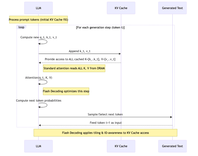
Flash Decoding applies FlashAttention principles here:

It fetches blocks of keys and values from the KV cache (likely in DRAM) into SRAM.
Computes attention against the current query $q_t$ using the tiling and on-chip accumulation methods.
Efficiently handles the causal masking needed for autoregressive generation.

7.2 Real-world Inference Gains

This optimization directly translates to faster text generation:

1.5–2.0× speedups (or more) in tokens-per-second for typical sequence lengths (1K–4K).
Lower memory bandwidth usage during inference, allowing larger batch sizes or deployment on less powerful GPUs.
Improved GPU utilization, as the chip spends less time waiting for data from the KV cache.

For production systems serving large language models, these inference speedups are critical for reducing latency and operational costs.

8. Inside FlashAttention: Conceptual Implementation

The real CUDA code is intricate, optimized down to the metal. But this Python-esque pseudocode gives a flavor of the core forward pass logic:

# Simplified conceptual pseudocode
def flash_attention_forward(Q, K, V, block_size_B=64):
    # Q, K, V assumed to be [batch, heads, N, head_dim] in DRAM
    N, head_dim = Q.shape[-2], Q.shape[-1]
    O = zeros_like(Q)  # Output buffer in DRAM
    scaling = 1.0 / sqrt(head_dim)
    
    # Iterate through blocks of the output sequence (rows of the conceptual N x N matrix)
    for i in range(0, N, block_size_B):
        # --- Load block of Queries into SRAM ---
        Qi = Q[:, :, i:i+block_size_B, :]  # Shape [B, h, B, d_k]
        
        # --- Initialize SRAM buffers for this query block ---
        Oi_block = zeros_like(Qi)        # Accumulator for output
        li_block = zeros([Q.shape[0], Q.shape[1], block_size_B]) # Accumulator for softmax denominator (log-sum-exp)
        mi_block = ones([Q.shape[0], Q.shape[1], block_size_B]) * (-infinity) # Running max for numerical stability

        # Iterate through blocks of the input sequence (columns of the conceptual N x N matrix)
        for j in range(0, N, block_size_B):
            # --- Load blocks of Keys and Values into SRAM ---
            Kj = K[:, :, j:j+block_size_B, :] # Shape [B, h, B, d_k]
            Vj = V[:, :, j:j+block_size_B, :] # Shape [B, h, B, d_v]
            
            # --- Compute attention scores for Qi and Kj block (in SRAM) ---
            Sij = matmul(Qi, transpose(Kj)) * scaling # Shape [B, h, B, B]
            
            # --- Update running statistics (in SRAM/registers) ---
            mi_block_old = mi_block
            mi_block_new = maximum(mi_block_old, reduce_max(Sij, axis=-1)) # Max score per query row in block

            # Calculate probabilities for current block, correcting for new max
            Pij = exp(Sij - mi_block_new.unsqueeze(-1)) # Numerically stable exp

            # Update denominator accumulator, rescaling previous value
            li_block_new = (li_block * exp(mi_block_old - mi_block_new) + 
                            reduce_sum(Pij, axis=-1))

            # --- Update output accumulator (in SRAM), rescaling previous value ---
            Oi_block_new = (Oi_block * exp(mi_block_old - mi_block_new).unsqueeze(-1) +
                            matmul(Pij, Vj)) # Pij * Vj

            # Update stats for next iteration
            mi_block = mi_block_new
            li_block = li_block_new
            Oi_block = Oi_block_new
            
        # --- Write final results for this query block back to DRAM ---
        O[:, :, i:i+block_size_B, :] = Oi_block / li_block.unsqueeze(-1) # Normalize output
        
    return O

This captures the essence: load blocks, compute locally in fast memory, accumulate statistics, update output, repeat, all while avoiding the formation of the full $N \times N$ matrix in slow memory.

9. Future Directions and Research Frontiers

FlashAttention wasn’t an endpoint; it was a catalyst. It opened doors and pointed the way for further research:

9.1 Scaling to Extremes

The ability to handle longer sequences efficiently fuels research into:

Massive Context Windows: Models capable of processing 100K, 1M, or even more tokens, enabled by FlashAttention variants.
Efficient Long-Sequence Architectures: Combining FlashAttention with techniques like sliding window attention or hierarchical methods for document-level understanding.

9.2 Algorithm-Hardware Co-Design

The success of FlashAttention underscores the need to design algorithms with hardware realities in mind, leading to:

Attention-Specific Hardware: GPUs or accelerators with architectural features explicitly designed to optimize attention patterns (e.g., specialized memory paths, matrix units).
Hardware-Aware Libraries: Software libraries that can automatically select the most efficient attention implementation based on the underlying hardware.

9.3 Beyond Text

The efficiency gains are valuable wherever Transformers are used:

Vision: Handling high-resolution images efficiently in Vision Transformers (ViTs).
Audio & Speech: Processing long audio streams for transcription or generation.
Multimodal Models: Optimizing the costly cross-attention layers that connect different data types (like text and images).

10. Conclusion: The FlashAttention Revolution

FlashAttention fundamentally changed how we approach Transformer efficiency. By identifying and attacking the memory IO bottleneck – a constraint often overshadowed by the pursuit of raw FLOPS – it delivered a potent combination of benefits:

Mathematically Exact Attention: No loss in model quality, unlike approximation methods.
Radical Memory Reduction: Often 2-3x or more, unlocking longer sequences and larger batches.
Significant Speedups: 2x or greater improvements in both training and inference.
Enabling the Impossible: Making previously infeasible long-context models practical.
Synergy: Amplifying gains when used alongside other fused kernel optimizations.

More profoundly, FlashAttention serves as a powerful reminder that clever algorithmic design, deeply informed by hardware constraints, can yield breakthroughs as significant as architectural innovations. It championed the importance of memory-aware algorithms and algorithm-hardware co-design. As AI models continue their relentless growth in scale and complexity, the principles pioneered by FlashAttention will be indispensable for sustainable progress. Its techniques are now baked into core deep learning libraries, silently powering many of the most advanced AI systems we use today, a testament to its foundational impact.

References and Further Reading

Tri Dao et al. (2022), “FlashAttention: Fast and Memory-Efficient Exact Attention with IO-Awareness.” arXiv:2205.14135
Tri Dao et al. (2023), “FlashAttention-2: Faster Attention with Better Parallelism and Work Partitioning.” arXiv:2307.08691
FlashAttention GitHub Repository: HazyResearch/flash-attention
xFormers Library: facebookresearch/xformers – Includes various memory-efficient attention implementations.
Megatron-LM: NVIDIA/Megatron-LM – Large model training framework often incorporating optimized kernels.
Efficiently Scaling Transformer Inference (DeepMind): arXiv:2211.05102 (Discusses inference bottlenecks)

Posted in AI / ML, LLM Advanced, LLM Research by Rakshit Kalra