Training Compute-Optimal Large Language Models: The Chinchilla Paradigm
1. Introduction
In March 2022, DeepMind published their groundbreaking paper introducing Chinchilla, which fundamentally changed our understanding of optimal LLM training strategies. The paper presented a critical insight that has since reshaped the field:
For a fixed compute budget, training a smaller model on more data yields better performance than training a larger model on less data.
This finding revealed that many prominent language models at the time (including early GPT-3 variants) were significantly undertrained relative to their parameter counts. The Chinchilla research refined our understanding of scaling laws by providing concrete guidelines for balancing model size against training data volume under fixed computational constraints.
This article explores:
- The mathematical foundation of compute-optimal scaling.
- How Chinchilla’s findings relate to established power-law scaling observations.
- Practical considerations for implementing compute-optimal training.
- Advanced techniques including epoch planning, curriculum learning, and distributed training.
2. The Compute-Optimal Equation and Its Implications
2.1 The Core Equation
The central contribution of the Chinchilla paper was a formula describing the optimal relationship between model size and training data. In simplified form, we can express this as:
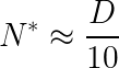
Where: –  = The optimal number of parameters (in billions) –
  = The total training tokens (in billions)
This represents a crucial shift from earlier scaling laws, suggesting that for optimal performance, your model should have approximately 20 billion parameters for every 200 billion tokens of training data (a 1:10 ratio).
The more general form accounting for compute budget is:
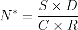
Where: – = Optimal parameter count –  = Size of training dataset (total tokens) – = Factor capturing training passes (epochs × batch size × steps) –
  = Total compute budget (typically measured in FLOPs) –
  = Ratio accounting for training vs. inference compute allocation
2.2 Key Insights from the Formula
- Balanced Scaling: Both model size and training data should scale proportionally with available compute.
- The 1:10 Rule of Thumb: For every parameter in your model, you should train on approximately 10 tokens of data. This contrasts with previous approaches that favored parameter count over training data volume.
- Compute-Efficiency Tradeoff: The formula quantifies how to maximize performance given your computational constraints, leading to more efficient resource allocation.
- Diagnosing “Undertrained” Models: Many early large language models had far more parameters than their training data could effectively utilize—Chinchilla identified this inefficiency and provided a correction.
3. Understanding Power-Law Scaling in Language Models
3.1 The Mathematics of Scaling Laws
Before Chinchilla, scaling laws were often expressed using power-law relationships of the form:

Where: –  = Loss (prediction error) –
  = Number of parameters – = Training dataset size (tokens) –
  and
and  = Power-law exponents –
  ,
,  , and = Constants
Kaplan et al. (2020) established that both model size and dataset size followed power-law relationships with model performance, but didn’t fully address the optimal balance between them.
3.2 Chinchilla’s Refinement of Scaling Laws
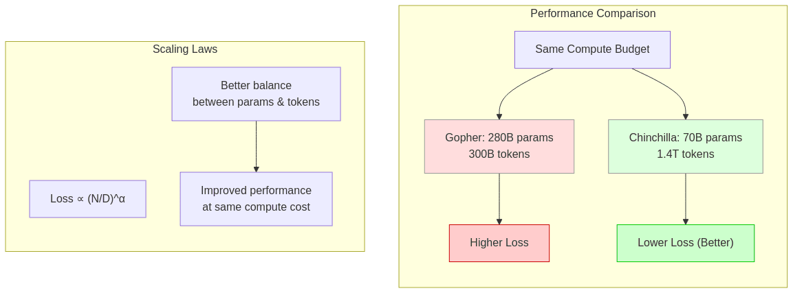
Chinchilla refined these observations by demonstrating that the relationship between loss, model size, and data is better described as:

This formula elegantly captures the insight that loss depends on the ratio between parameters and training tokens, not just their absolute values. When this ratio is imbalanced (specifically, when N is too large relative to D), you encounter diminishing returns—essentially wasting computational resources.
3.3 Empirical Evidence
The Chinchilla researchers demonstrated their theory by training a 70B parameter model (Chinchilla) on 1.4T tokens, which outperformed Gopher, a 280B parameter model trained on only 300B tokens, despite using the same compute budget. This provided compelling evidence that the field had been systematically overemphasizing parameter count at the expense of training data.
4. Practical Implementation Considerations
4.1 Determining Optimal Epoch Count
An epoch represents one complete pass through the entire training dataset. The Chinchilla findings have important implications for epoch planning:
- Single-Epoch Training: With very large datasets (trillions of tokens), a single epoch may be sufficient and aligns with the Chinchilla ratio.
- Multi-Epoch Training: When working with smaller datasets, multiple epochs may be necessary to reach the optimal token-to-parameter ratio. However, care must be taken to avoid overfitting.
- Compute vs. Data Tradeoff: When data is limited, you face a choice between:
- Training a smaller model that adheres to the Chinchilla ratio with available data
- Training a larger model for fewer steps (effectively reducing the tokens-per-parameter ratio)
Recent research suggests that slightly undertrained larger models may outperform perfectly balanced smaller models in some scenarios, but this remains an active area of research.
4.2 Curriculum Training Strategies
Curriculum learning involves structuring the training process to progressively increase in difficulty, similar to how human education is organized.
Types of Curriculum Approaches:
- Difficulty-Based Curriculum: Ordering training data from simplest to most complex examples
- For language models, this might mean starting with simple, grammatical text before introducing more complex or domain-specific content
- Quality-Based Curriculum: Beginning with high-quality, curated data before introducing noisier web-scraped content
- Many recent LLMs start with books and carefully filtered content before moving to broader internet data
- Domain-Progressive Curriculum: Gradually expanding the domains or topics covered during training
- For example, starting with general knowledge before introducing specialized scientific or technical content
Implementation Considerations:
- Dataset Preparation: Creating a curriculum requires careful data tagging and sorting.
- Dynamic Curricula: More advanced approaches adjust the curriculum based on the model’s learning progress.
- Compute Efficiency: Well-designed curricula can improve sample efficiency, potentially reducing the total tokens needed.

4.3 Distributed Training Techniques
Training compute-optimal models often requires advanced distributed computing strategies:
Fully Sharded Data Parallel (FSDP)
- The Challenge: Large models may not fit in a single GPU’s memory, especially when accounting for optimizer states and gradients
- How FSDP Works: Parameters, gradients, and optimizer states are sharded (divided) across multiple GPUs
- Implementation: During the forward and backward passes, each GPU temporarily gathers the parameters it needs
- Memory Efficiency: This approach can reduce per-GPU memory requirements by factors proportional to the number of devices
Other Parallel Training Strategies:
- Pipeline Parallelism: Divides the model’s layers across multiple devices
- Tensor Parallelism: Splits individual operations across devices
- 3D Parallelism: Combines data, pipeline, and tensor parallelism for maximum scalability
- Zero Redundancy Optimizer (ZeRO): Progressively eliminates memory redundancies in distributed training
Practical Considerations:
- Communication Overhead: Sharding introduces additional device-to-device communication
- Framework Support: Libraries like PyTorch FSDP, DeepSpeed, and Megatron-LM provide implementations
- Hardware Requirements: Different approaches have different GPU interconnect bandwidth requirements

5. Real-World Application Examples
5.1 Case Study: Applying Chinchilla Scaling to a 13B Parameter Model
Let’s walk through a practical example:
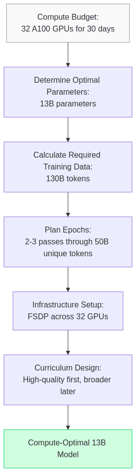
- Compute Budget Assessment:
- Suppose you have access to 32 A100 GPUs for 30 days
- This translates to approximately 10^23 FLOPs of compute
- Optimal Parameter Count:
- Following Chinchilla’s formula, you determine 13B parameters is optimal
- Required Training Data:
- The 1:10 ratio suggests you need approximately 130B tokens
- Your dataset contains 50B unique tokens, so you plan for 2-3 epochs
- Infrastructure Setup:
- Implement FSDP across your 32 GPUs to efficiently distribute the model
- Set up checkpointing every 1000 steps to enable training resumption
- Curriculum Design:
- First epoch: high-quality curated corpus
- Subsequent epochs: broader web and domain-specific data
This approach ensures you’re maximizing your compute investment by following compute-optimal scaling principles.
5.2 Adapting to Resource Constraints
Not everyone has access to supercomputer-level resources. Here’s how to adapt Chinchilla principles at different scales:
- Limited Compute: Use a smaller model with proportionally less data
- Limited Quality Data: Consider multiple epochs on high-quality data rather than single-pass training on noisy data
- Time Constraints: Use pretrained smaller models and Chinchilla-optimal fine-tuning
6. Emerging Research and Future Directions
6.1 Beyond Text: Multimodal Scaling Laws
Researchers are now investigating whether Chinchilla-like scaling principles apply to:
- Image-Text Models: How do parameters scale with image-text pairs?
- Video Understanding: Do temporal sequences require different scaling considerations?
- Audio and Speech: What is the optimal token representation for audio data?
Early results suggest similar principles may apply, but with domain-specific adjustments.
6.2 Specialized Architectures and Efficient Training
Several innovations are enhancing compute-optimal training:
- Mixture-of-Experts (MoE): These architectures may offer different scaling properties by activating only a subset of parameters per token.
- Flash Attention: Reducing the computational cost of attention mechanisms.
- Quantization-Aware Training: Training models with lower precision from the start.
6.3 Transfer Learning and Foundation Models
The relationship between pretraining and fine-tuning continues to evolve:
- Chinchilla for Fine-tuning: How do these scaling laws apply when adapting pretrained models?
- Domain-Specific Scaling: Do specialized domains require different parameter-to-token ratios?
- Instruction Tuning Efficiency: Can Chinchilla principles improve the efficiency of RLHF and instruction tuning?
7. Conclusion
The Chinchilla research represents a fundamental shift in how we approach language model training. By establishing that many models were dramatically undertrained relative to their size, DeepMind provided a clear blueprint for more efficient resource allocation.
The key takeaways:
- Balance is Critical: The ratio between parameters and training tokens matters more than maximizing either in isolation.
- Compute-Optimality: For a fixed compute budget, follow the Chinchilla formula to maximize performance.
- Practical Implementation: Advanced techniques like curriculum learning and distributed training are essential for applying these principles at scale.
- Ongoing Evolution: The field continues to refine these relationships as we explore multimodal learning and specialized architectures.
By adhering to these principles, researchers and organizations can develop more capable language models while using computational resources more efficiently—a crucial consideration as models continue to grow in scale and capability.
References
- Hoffmann et al. (2022): “Training Compute-Optimal Large Language Models” – The original Chinchilla paper
- Kaplan et al. (2020): “Scaling Laws for Neural Language Models” – Early work on power-law scaling
- Bengio et al. (2009): “Curriculum Learning” – Foundational work on curriculum learning
- PyTorch FSDP Documentation: FullyShardedDataParallel – Technical details on implementing FSDP
- Brown et al. (2020): “Language Models are Few-Shot Learners” – GPT-3 paper showing pre-Chinchilla scaling
- Chowdhery et al. (2022): “PaLM: Scaling Language Modeling with Pathways” – Google’s approach to scaling
- Touvron et al. (2023): “LLaMA: Open and Efficient Foundation Language Models” – Meta’s implementation of efficient scaling
This article was last updated in November 2023 to reflect the latest developments in compute-optimal language model training.