1. Introduction
Deep learning loves its floating-point numbers. float32 is the default, the comfortable standard where models are born and trained. It offers precision, a vast dynamic range – a safety net for complex gradients and subtle weight updates. But this comfort comes at a cost. As models balloon, packing billions, even trillions, of parameters, that float32 luxury turns into a crushing weight – demanding absurd amounts of memory, compute power, and energy.
Enter quantization. It’s not elegant. It’s not theoretically pure. It’s the pragmatic, often brutal, act of taking those high-precision numbers and forcing them into smaller, less expressive formats – like 8-bit integers (int8) or even cruder 4-bit representations. Think of it as lossy compression for neural networks.
Why bother with this numerical butchery? Survival. Deploying gargantuan models onto phones, edge devices, or even just cost-effective servers demands ruthless efficiency. Quantization is about making these powerful models actually usable in the real world, trading some numerical fidelity for massive gains in size, speed, and power efficiency. Let’s dissect how it works, why it matters, and the unavoidable tradeoffs.
2. Understanding Numerical Precision in Deep Learning
Before we chop things up, let’s understand the building blocks we’re starting with.
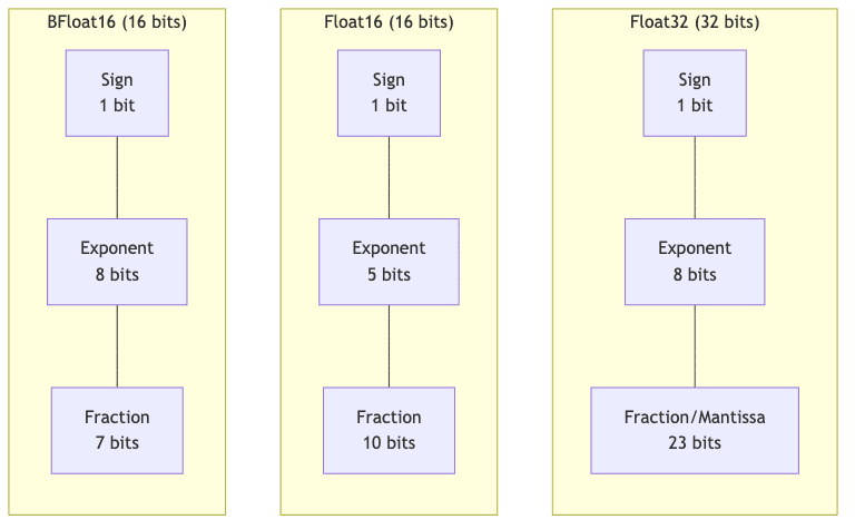
2.1 Floating-Point Formats
- Float32 (Single Precision)
- Bit allocation: 1-bit sign, 8-bit exponent, 23-bit fraction (mantissa)
- Memory: 32 bits (4 bytes) per parameter – the heavyweight champion.
- Dynamic range: Huge (approx. ±1.18 × 10^-38 to ±3.4 × 10^38).
- Usage: The default training ground. Reliable, forgiving, but memory-hungry.
- Float16 (Half Precision)
- Bit allocation: 1-bit sign, 5-bit exponent, 10-bit fraction (mantissa)
- Memory: 16 bits (2 bytes) – half the size, double the potential speedup (sometimes).
- Dynamic range: Much smaller (approx. ±6.10 × 10^-5 to ±65,504). Prone to underflow/overflow issues if not handled carefully.
- Usage: Common in mixed-precision training on modern GPUs. Faster, leaner, but requires vigilance against numerical instability.
- BFloat16 (Brain Floating Point)
- Bit allocation: 1-bit sign, 8-bit exponent, 7-bit fraction
- Memory: 16 bits (2 bytes) – same size as FP16.
- Advantage: Keeps the wide dynamic range of FP32 (same 8-bit exponent) but sacrifices fraction precision. More stable than FP16 for training deep models.
- Usage: Google’s pragmatic child, now widely adopted in AI hardware for training and inference. A good compromise.
Moving down this ladder changes the fundamental arithmetic. The trick is to harness the efficiency gains without letting the reduced precision cripple the model’s intelligence.
3. What Is Quantization?
At its core, quantization maps a continuous range of high-precision values (like float32) onto a discrete, smaller set of low-precision values (like int8). It’s about approximation.
- Weights and activations, the lifeblood of the network, get converted.
- This conversion relies on scale factors (how much to stretch or shrink the original range) and often zero-point offsets (what low-precision value represents true zero). These parameters try to capture the essence of the original distribution.
- The result: numbers that need fewer bits, meaning smaller models and potentially much faster math operations, especially on specialized hardware.
The core quantization formula for simple linear quantization looks like this:
Where:
is the resulting quantized integer (e.g., clamped between 0 and 255 for
uint8).is the original
float32value.is the scale factor (float).
is the zero-point (integer), mapping the floating-point zero to an integer value.
To get an approximation back (dequantization):
Yes, this introduces rounding errors – a slight fuzziness. But neural networks, particularly large ones, often possess a surprising resilience to this kind of noise, if the quantization is done smartly.
4. Why Quantization Matters: The Practical Benefits
Why embrace this seemingly crude approximation? Because the practical wins can be enormous.
4.1 Memory Efficiency
- Model size reduction: The most obvious win. An
int8model is 4x smaller than itsfp32parent (8 bits vs 32 bits). A 4-bit model? 8x smaller. - Example: That cutting-edge 7B parameter LLM needing ~28GB in
fp32? Quantize it toint8, and suddenly it fits into ~7GB, potentially runnable on a decent consumer GPU, not just a data center rack. - Storage & Distribution: Smaller models are easier to download, store on edge devices with limited flash memory, and push over networks.
4.2 Computation Speed
- Reduced memory bandwidth: Often the real bottleneck isn’t raw compute power, but shuffling data between memory and the processor. Lower precision means less data to move for every operation. Less data = faster execution.
- Hardware acceleration: Modern CPUs (AVX, VNNI), GPUs (Tensor Cores), and dedicated AI chips (TPUs, NPUs) have specialized instructions that crunch low-precision integer math much faster (often 2-4x or more) than floating-point.
- Batch throughput: Smaller memory footprint means you can potentially fit larger batches into GPU memory, improving overall throughput in inference servers.
4.3 Energy Efficiency
- Power consumption: Moving data costs energy. Less data movement and faster, simpler integer operations mean lower power draw.
- Mobile and edge deployment: Absolutely critical for battery-powered devices. Quantization can slash energy use, extending device life.
- Data center implications: At hyperscale, even small percentage reductions in power per inference translate into massive savings on electricity bills and cooling costs. It’s greener, too (or less destructive, anyway).
4.4 Real-world Performance Preservation
- This is the tightrope walk. Miraculously,
int8quantization, when done well (using calibration data), often results in accuracy drops of less than 1% compared to thefp32baseline. - Aggressive 4-bit quantization might cost 1-3% accuracy but offers huge efficiency gains, often acceptable depending on the application.
- You can strategically choose what to quantize, leaving sensitive parts of the model in higher precision.
5. Types of Quantization
There isn’t just one way to quantize. The main approaches differ in when you do it and how you map the numbers.
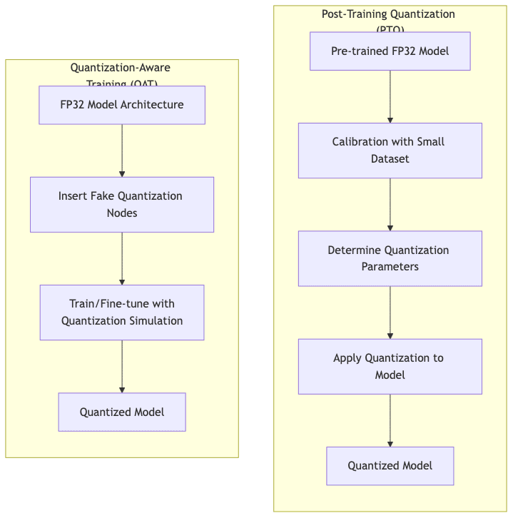
5.1 Post-Training Quantization (PTQ)
- Process: Take a pre-trained
fp32model and convert it after training is complete. - Calibration: Usually involves feeding a small, representative dataset through the model to observe the ranges of weights and activations, helping determine optimal scale/zero-point values.
- Advantages:
- Simple, fast – no retraining needed.
- Widely supported by frameworks and tools.
- The “quick fix” approach.
- Limitations:
- Accuracy can suffer, especially for ultra-low precision (<8 bits). The model wasn’t trained with quantization noise in mind.
- Can struggle with models having bizarre activation distributions.
5.2 Quantization-Aware Training (QAT)
- Process: Simulate the effects of quantization during the training (or fine-tuning) process. Insert “fake” quantization nodes into the model graph.
- Training modifications: The forward pass uses quantized weights/activations (simulating inference), but the backward pass uses full-precision gradients to allow stable learning. The model learns to compensate for quantization noise.
- Advantages:
- Generally yields higher accuracy, especially for aggressive quantization (4-bit, etc.).
- The model becomes inherently robust to the quantization process.
- Limitations:
- Requires (re)training or significant fine-tuning – computationally expensive.
- More complex to set up and implement correctly.
5.3 By Numerical Format
5.3.1 Integer Quantization
- INT8: The workhorse. Best balance of efficiency and accuracy for most use cases. Widely supported by hardware.
- INT4/INT2: Extreme compression, pushing the limits. Requires sophisticated techniques (often QAT, careful calibration) to maintain usable accuracy.
- Asymmetric vs. Symmetric:
- Asymmetric: Uses both scale (
- Symmetric: Assumes the distribution is centered around zero, uses only scale (
. Simpler math, sometimes slightly less accurate but often faster on hardware.
- Asymmetric: Uses both scale (
5.3.2 Low-Bit Floating Point
- FP8: A newer contender, aiming for a middle ground. Comes in flavors like E4M3 (more precision, less range) and E5M2 (more range, less precision) tailored for different parts of a network. Supported by latest-gen GPUs.
- FP4: Even more aggressive. Formats like NF4 (NormalFloat4) used in libraries like
bitsandbytesare cleverly designed to handle the distributions common in large transformers. - Advantage: Can handle outliers and wider dynamic ranges better than low-bit integers, potentially preserving more accuracy in tricky layers.
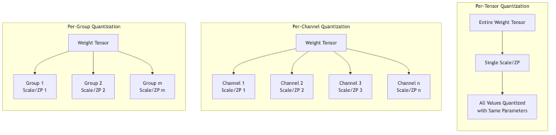
5.4 By Granularity
How widely are the scale/zero-point factors applied?
5.4.1 Per-Tensor Quantization
- One single scale/zero-point pair for an entire weight tensor (e.g., all weights in a convolutional layer).
- Simplest, lowest overhead. Can be inaccurate if values within the tensor vary wildly.
5.4.2 Per-Channel Quantization
- Different scale/zero-point for each output channel in a convolutional filter, or each row/column in a linear layer.
- Much better at preserving accuracy, especially for CNNs, as it adapts to variations across channels.
- Slightly more overhead to store/manage multiple scale/zero-point values.
5.4.3 Per-Group Quantization
- A compromise. Group channels (e.g., groups of 64 or 128) and assign a scale/zero-point per group.
- Balances accuracy and overhead. Common in modern LLM quantization (like GPTQ).
6. Quantization Techniques in Practice
The basic math is simple, but real-world quantization often requires more sophisticated tricks.
6.1 Simple Linear Quantization Example
A basic recipe for uniform uint8 (unsigned 8-bit integer) quantization:
# Find min/max values from calibration data or weights
min_val = tensor.min().item()
max_val = tensor.max().item()

# Asymmetric quantization (uint8: range 0-255)
scale = (max_val - min_val) / 255.0
zero_point = round(-min_val / scale) # Integer zero point

# Quantize a value x
quant_val = round(x / scale) + zero_point
quant_val = max(0, min(quant_val, 255)) # Clamp to range
For symmetric int8 (signed 8-bit integer, range typically -127 to 127):
# Find max absolute value
max_abs = max(abs(min_val), abs(max_val))

# Symmetric quantization (int8: range -127 to 127)
scale = max_abs / 127.0
zero_point = 0 # Fixed zero point for symmetric

# Quantize a value x
quant_val = round(x / scale)
quant_val = max(-127, min(quant_val, 127)) # Clamp to range
6.2 Advanced Techniques
Simple methods often hit limits. Here’s where things get more clever:
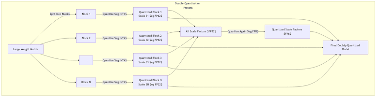
6.2.1 Double Quantization
Storing per-channel or per-group scale factors can itself become a memory burden for huge models. Double Quantization tackles this:
- Quantize the main weights, typically per-block or per-group, generating many scale factors.
- Collect these scale factors.
- Quantize the scale factors themselves to an even lower precision (e.g., FP8 or INT8).
This adds a second layer of compression, reducing the metadata overhead. Used effectively in libraries like bitsandbytes.
6.2.2 Outlier-Aware Quantization
A few extreme values (outliers) in weights or activations can wreck quantization. They force the scale factor to cover a huge range, crushing the precision for the vast majority of ‘normal’ values. Solutions:
- Identify outliers: Find values beyond a certain threshold (e.g., multiple standard deviations).
- Mixed Precision for Outliers: Keep the outliers in
fp16orfp32while quantizing the rest toint8/int4. Requires specialized handling during computation. - Clipping: Simply cap the extreme values at a threshold before calculating scale/zero-point. Loses information in the outliers but improves precision for the rest.
6.2.3 Mixed-Precision Quantization
Why force the entire network into int8 or int4 if only some layers can tolerate it?
- Sensitivity Analysis: Profile the model to see which layers suffer most from quantization (often the first and last layers, or layers with critical normalization steps).
- Selective Application: Apply aggressive quantization (
int4) to robust layers (e.g., large linear layers in transformers) and keep sensitive layers at higher precision (int8,fp16, or evenfp32). - Requires careful balancing and framework support, but often achieves the best accuracy/performance tradeoff.
7. Hardware Considerations and Acceleration
Quantization’s real value is unlocked by hardware designed to exploit it.
7.1 Hardware Support
- CPUs:
- Modern x86 chips (Intel, AMD) have instructions like VNNI and AVX-512 specifically for accelerating
int8operations. - ARM cores (common in mobile/edge) often include specialized dot-product instructions for
int8/int4.
- Modern x86 chips (Intel, AMD) have instructions like VNNI and AVX-512 specifically for accelerating
- GPUs:
- NVIDIA’s Tensor Cores are beasts at low-precision math, supporting
int8,int4,fp8, and binary/ternary operations with massive speedups. - AMD GPUs also incorporate low-precision matrix acceleration features.
- NVIDIA’s Tensor Cores are beasts at low-precision math, supporting
- Specialized Accelerators:
- Google TPUs are heavily optimized for
bf16andint8. - Dedicated AI chips from Qualcomm, Apple, MediaTek etc., often prioritize quantized integer performance for power efficiency on edge devices.
- Google TPUs are heavily optimized for
7.2 Framework Support
You need software tools to actually do the quantization.
- PyTorch: Has robust quantization tools (
torch.quantization, FX Graph Mode Quantization) supporting PTQ (static, dynamic) and QAT. - TensorFlow: TF Lite is the primary vehicle for deploying quantized models, especially on mobile and edge.
- ONNX Runtime: Provides cross-platform quantization capabilities and optimized execution backends for various hardware.
- Specialized Libraries:
bitsandbytes: Focuses on efficient 4-bit, 8-bit, and double quantization for large transformers.- GPTQ, AutoGPTQ: Implementations of the GPTQ algorithm for post-training quantization of LLMs.
- Apache TVM: A compiler framework that can optimize and quantize models for specific hardware targets.
8. Implementation Example: PyTorch Quantization
Here’s a taste of how PTQ looks in PyTorch.
import torch
import torch.nn as nn
import os
from torch.quantization import get_default_qconfig, quantize_jit, prepare_jit, convert

# Assume 'model' is your pre-trained nn.Module model
# Assume 'calibration_loader' is a DataLoader with representative data

def ptq_static_example(model, calibration_loader):
    model.eval()

    # Choose quantization configuration based on target
    # 'fbgemm' for x86 server, 'qnnpack' for ARM mobile
    qconfig = get_default_qconfig('fbgemm')
    model.qconfig = qconfig

    # Fuse modules like Conv+BN+ReLU for better quantization compatibility
    # Example: torch.quantization.fuse_modules(model, [['conv1', 'bn1', 'relu1']], inplace=True)
    # (Requires specific model structure knowledge)

    print("Preparing model for static quantization...")
    # Insert observers to collect activation statistics
    model_prepared = torch.quantization.prepare(model, inplace=False)

    print("Calibrating...")
    # Run calibration data through the prepared model
    with torch.no_grad():
        for input_data, _ in calibration_loader:
             # Move data to appropriate device if needed
            model_prepared(input_data) # This collects stats

    print("Converting to quantized model...")
    # Convert the model, replacing modules and using collected stats
    quantized_model = torch.quantization.convert(model_prepared, inplace=False)

    # Optional: Script the model for deployment
    scripted_quantized_model = torch.jit.script(quantized_model)

    # Verify size reduction
    torch.jit.save(torch.jit.script(model.cpu()), "fp32_model.pt") # Save original scripted
    torch.jit.save(scripted_quantized_model.cpu(), "int8_model_static.pt")
    fp32_size = os.path.getsize("fp32_model.pt") / (1024 * 1024)
    int8_size = os.path.getsize("int8_model_static.pt") / (1024 * 1024)

    print(f"FP32 Model size: {fp32_size:.2f} MB")
    print(f"INT8 Model size: {int8_size:.2f} MB")
    if int8_size > 0:
        print(f"Compression ratio: {fp32_size/int8_size:.2f}x")
    else:
         print("INT8 model size is zero or invalid.")


    return scripted_quantized_model

# Example Usage (requires a defined model and calibration_loader)
# dummy_model = nn.Sequential(nn.Conv2d(3, 32, 3), nn.ReLU(), nn.Linear(26*26*32, 10)) # Example model
# dummy_data = [(torch.randn(1, 3, 28, 28), torch.tensor([1])) for _ in range(10)] # Example data
# quantized_scripted_model = ptq_static_example(dummy_model, dummy_data)
For more fine-grained control, especially with complex models or per-channel needs, FX Graph Mode Quantization is often preferred:
import torch
import torch.quantization.quantize_fx as quantize_fx
# Assume 'model' and 'calibration_loader' are defined

def fx_graph_mode_ptq(model, calibration_loader):
    model.eval()

    # Define quantization configuration mapping
    # Can specify different configs for different module types or names
    qconfig_mapping = quantize_fx.get_default_ptq_qconfig_mapping()
    # Example customization: use per-channel for Linear layers
    # qconfig_mapping.set_module_name("fc_layer_name", torch.quantization.get_default_qconfig('fbgemm')) # Example specific layer


    print("Preparing model with FX Graph Mode...")
    # Automatically traces the model and inserts observers
    model_prepared = quantize_fx.prepare_fx(model, qconfig_mapping, example_inputs=torch.randn(1, 3, 28, 28)) # Provide example input shape

    print("Calibrating...")
    with torch.no_grad():
        for input_data, _ in calibration_loader:
            model_prepared(input_data) # Collect stats

    print("Converting model...")
    # Converts the prepared model to a quantized version
    quantized_model = quantize_fx.convert_fx(model_prepared)

    # Optional: Scripting for deployment
    # scripted_quantized_model = torch.jit.script(quantized_model)
    # (May require handling FX-specific constructs if scripting)

    # Size verification similar to previous example...

    return quantized_model

# Example Usage
# quantized_fx_model = fx_graph_mode_ptq(dummy_model, dummy_data)
(Note: The provided code snippets are illustrative. Real-world usage requires careful setup of models, data loaders, and potentially module fusion or custom configuration.)
9. Quantization for Different Model Types
Different architectures have different sensitivities.
9.1 Convolutional Neural Networks (CNNs)
- Generally robust candidates for
int8quantization. Often see minimal accuracy loss with PTQ. - Convolutional layers benefit significantly from per-channel quantization.
- Common wisdom: The first (input) and last (output/classifier) layers are sometimes more sensitive. May benefit from keeping them at
fp16orfp32(mixed precision).
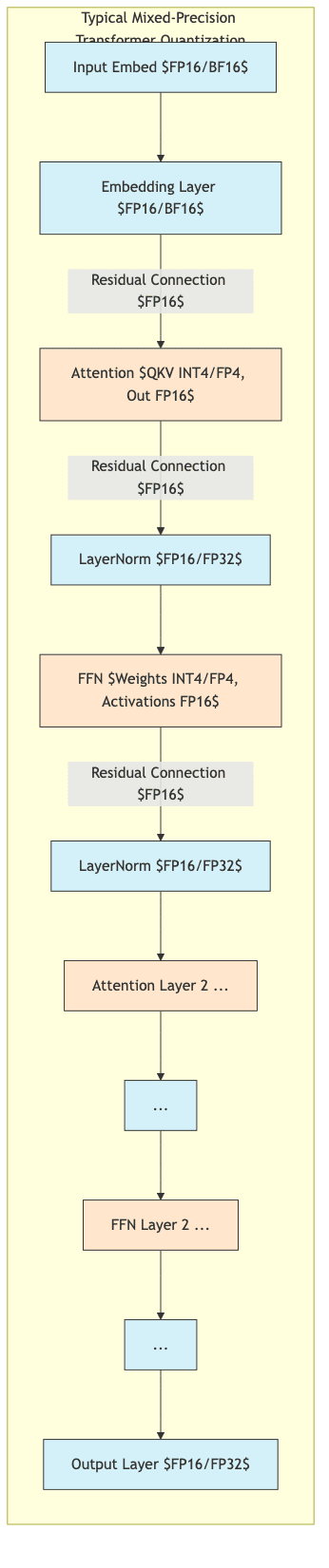
9.2 Transformers and Large Language Models (LLMs)
- The tricky ones. Attention mechanisms and Layer Normalization can be sensitive.
- Weight distributions often have significant outliers, problematic for simple quantization.
- Effective strategies often involve:
- Mixed Precision: Keep embeddings, LayerNorm, and output layers at higher precision (
bf16/fp16). - Outlier Handling: Use techniques like outlier-aware quantization or specialized formats (
NF4,FP4) for the large weight matrices in attention and FFN layers. - Per-Group/Per-Channel: Essential for dense layers to capture variations.
- Specialized libraries (
bitsandbytes,GPTQ) are often necessary for state-of-the-art LLM quantization.
- Mixed Precision: Keep embeddings, LayerNorm, and output layers at higher precision (
9.3 Recurrent Neural Networks (RNNs)
- The long chains of computation in RNNs (LSTMs, GRUs) can accumulate quantization errors over time steps.
- Sensitivity is high, especially in the recurrent state transitions.
- Mitigation strategies:
- Use higher precision (
int8orfp16) for the recurrent connections/gates. - QAT is often more effective than PTQ here.
- Techniques like layer-specific parameters or periodic state recalibration might be needed for very long sequences.
- Use higher precision (
10. Performance Benchmarks and Trade-offs
It’s always a balancing act. Here’s a rough guide:
10.1 Accuracy vs. Size vs. Speed
| Precision | Size Reduction (vs FP32) | Typical Accuracy Drop | Speed Improvement (Ideal Hardware) |
|---|---|---|---|
| FP16/BF16 | 2x | <0.1% – 0.5% | 1.3x – 2x |
| INT8 | 4x | 0.5% – 1.5% | 2x – 4x+ |
| INT4 | 8x | 1% – 5% | 3x – 8x+ |
| INT2/Binary | 16x – 32x | Highly variable (5%+) | Potentially 4x – 16x+ |
Disclaimer: Your mileage will vary significantly based on model, task, data, implementation quality, and specific hardware.
10.2 Where Quantization Works Best
- Large, overparameterized models: Lots of redundancy means more fat to trim without hitting bone.
- Transfer learning: Fine-tuned models often have excess capacity that quantization can exploit.
- Inference-focused deployments: No need to worry about stable training dynamics.
- Hardware with strong low-precision support: The speedups are real if the silicon is built for it.
10.3 When to Be Cautious
- Small, already highly optimized models: Less redundancy, less room for error.
- Tasks requiring extreme precision: Certain scientific simulations, maybe some high-fidelity perception tasks.
- Models dealing with rare events or long tails: Quantization can obscure subtle but important signals.
- Safety-critical domains: Requires extremely rigorous validation to ensure quantization doesn’t introduce unexpected failure modes. Don’t quantize your self-driving car’s perception model without knowing exactly what you’re doing.
11. Current Research and Future Directions
The field is constantly evolving as researchers push the boundaries of efficiency.
11.1 Emerging Techniques
- Vector Quantization (VQ): Grouping weights/activations and representing them by codes from a learned codebook.
- Learned Quantization Parameters: Using gradients or reinforcement learning to find optimal scale/zero-point values instead of simple heuristics.
- Binary/Ternary Networks: Extreme quantization where weights are just +1, 0, -1. Requires specialized training but offers maximum theoretical efficiency.
- Quantization + Parameter-Efficient Fine-Tuning (PEFT): Combining methods like LoRA with quantization for efficient adaptation and deployment (e.g., QLoRA).
11.2 Standardization Efforts
- Growing industry push to standardize formats like FP8 for better interoperability across hardware.
- Frameworks are making quantization easier, integrating it more deeply.
- More automated tools (AutoML for quantization) are emerging to find optimal strategies.
12. Practical Recommendations
So, you want to quantize your model? Some hard-earned advice:
- Start Simple: Try
int8PTQ first. It’s often good enough and sets a baseline. - Measure Everything: Don’t guess. Benchmark accuracy (on a relevant eval set), latency (on target hardware), model size, and memory usage before and after.
- Identify Bottlenecks: Profile your model. Which layers are most computationally expensive? Which are most sensitive to accuracy drops?
- Iterate Granularly: If uniform
int8isn’t cutting it, explore mixed precision. Quantize the robust parts aggressively, protect the sensitive ones. Use per-channel/per-group where needed. - Know Your Hardware: Optimize for the target platform’s capabilities.
int8on a CPU without VNNI might not be much faster thanfp32. - Calibrate Wisely: Use calibration data that truly reflects the distribution your model will see in production. Garbage in, garbage out applies to calibration too.
- Set Guardrails: Define acceptable accuracy degradation before you start. Don’t chase efficiency blindly off an accuracy cliff.
13. Conclusion
Quantization isn’t the most glamorous part of deep learning. It’s the gritty engineering required to bridge the gap between massive, power-hungry models trained in the cloud and practical applications running efficiently in the real world. It’s a concession to physics and economics.
As models inevitably continue their relentless march towards larger scale, quantization transforms from a mere optimization technique into a fundamental necessity. It’s no longer an afterthought but a core consideration for anyone serious about deploying AI.
The techniques are getting smarter, pushing towards 4-bit and lower precisions while clawing back accuracy through methods like QAT, outlier handling, and mixed precision. The future likely involves even tighter integration between architecture design and quantization, more standardization, and smarter automation.
For practitioners, understanding quantization—its methods, its benefits, and critically, its tradeoffs—is no longer optional. It’s part of the job of building AI that actually works, not just AI that looks good on a leaderboard.