Joint Embedding Predictive Architecture (JEPA): An Advanced Framework for Efficient AI Prediction and Decision-Making

1. Introduction: Escaping the Generative Bottleneck

The current AI zeitgeist seems obsessed with generative models. We’re building systems that paint stunning pictures, write plausible prose, even predict intricate environment states. The goal often appears to be mimicking reality with ever-increasing fidelity – reconstructing the world bit by byte, pixel by pixel. Think diffusion models, GANs, autoregressive behemoths.

On the other side, we have discriminative or energy-based models, systems focused on learning cost landscapes, assigning low energy (high desirability) to good states and high energy to bad ones. Useful, but often lacking the rich world understanding of their generative cousins.

Joint Embedding Predictive Architecture (JEPA) carves out a third path, a pragmatic rebellion against the inefficiencies of pure generation. It asks a fundamental question: Why waste colossal compute trying to predict every irrelevant detail of the world?

JEPA refuses the generative burden. It doesn’t try to reconstruct raw observations, sidestepping the often-intractable cost of modeling noise or inconsequential variations.
It learns rich latent representations, distilling the essence of the environment, but frames this learning within an energy-based optimization framework.

This hybrid strategy makes JEPA potent for complex decision-making. By shifting the prediction game to embedding spaces, JEPA drastically cuts the dimensionality of the problem while, crucially, retaining the information needed to act effectively. It’s about predicting what matters, not just what is.

2. Core Principles: The Machinery of Latent Prediction

JEPA isn’t magic; it’s an architecture built from interacting components designed for efficient foresight:

2.1 Key Components

Observation Space $x_t$ : The raw, often messy, input from the world at time t (an image, sensor feed, state vector).
Encoder $\text{Enc}(\cdot)$ : A neural network tasked with distilling the high-dimensional observation into a compact latent code: $s_t = \text{Enc}(x_t)$ where $s_t$ is the compressed essence, the latent state embedding.
Predictor $\text{Pred}(\cdot)$ : Projects the current understanding forward, forecasting the next latent state, potentially considering an action: $\hat{s}_{t+1} = \text{Pred}(s_t, a_t)$ $\hat{s}_{t+1}$ is the imagined future embedding given action $a_t$ .
Cost/Energy Module $\text{C}(\cdot)$ : The arbiter of desirability. Assigns a scalar cost or energy to latent states, lower values indicating preference: $E(s_t) = \text{C}(s_t)$ Or, more realistically, it considers the transition: $E(s_t, a_t, \hat{s}_{t+1}) = \text{C}(s_t, a_t, \hat{s}_{t+1})$ .
Actor $\text{A}(\cdot)$ : The decision-maker. Selects actions based on the latent state and the cost landscape, often guided by gradient descent: $a_t = \text{A}(s_t)$
Working Memory: A buffer to hold recent states, costs, or predictions, enabling multi-step reasoning and planning beyond immediate reflexes.

2.2 The JEPA Workflow: Thinking in Embeddings

The critical insight is where JEPA does its thinking. Instead of predicting the next frame of pixels, the cycle runs entirely in the latent space:

Distill the current observation $x_t$ into its essence $s_t$ .
Imagine the consequences: predict the future latent state $\hat{s}_{t+1}$ for potential actions.
Judge the outcomes: evaluate the cost/energy of these imagined future states.
Refine the plan: select or optimize actions to steer towards low-cost futures.
Act, observe the result, and repeat the cycle.

This focus allows JEPA to allocate compute where it counts – modeling the dynamics relevant for decisions, not recreating superficial details.

3. Perception-Action Paradigms: Reflex vs. Deliberation

JEPA isn’t monolithic; it supports different modes of operation, reflecting distinct approaches to the perception-action loop:

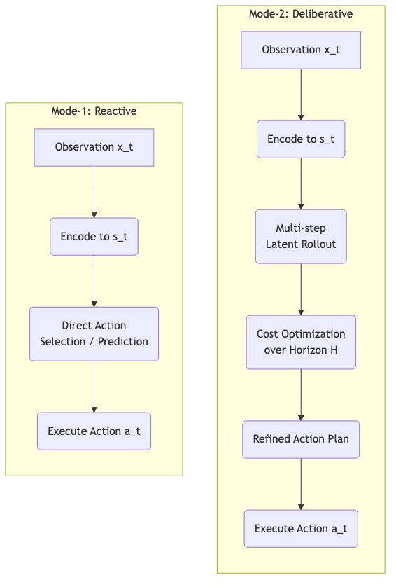
3.1 Mode-1: Reactive Perception-Action (The Reflex)

Here, JEPA acts quickly, almost instinctively:

Observe $x_t$ , encode to $s_t$ , generate action $a_t$ rapidly.
Prediction and cost evaluation are shallow, focused on the immediate next step.
The cost module weighs near-term consequences.
Speed and efficiency are paramount.

Think of scenarios demanding fast reactions, or where long-term prediction is futile due to chaotic dynamics.

3.2 Mode-2: Deliberative Perception-Action (The Planner)

Mode-2 embraces foresight, reasoning deeper into the future within the latent space:

Perform multi-step “imagination” rollouts: predict sequences $\hat{s}_{t+1}, \hat{s}_{t+2}, \ldots, \hat{s}_{t+H}$ over a horizon $H$ .
Optimize the entire action sequence to minimize the cumulative predicted cost: $\min_{a_0,\ldots,a_{H-1}} \sum_{t=0}^{H-1} \text{C}(\hat{s}_t, a_t, \hat{s}_{t+1})$
Iteratively refine predictions and the action plan before committing to the first step.
Enables sophisticated planning (robotics, strategy games, navigation) while remaining computationally feasible because the planning happens in the compressed latent space.

Mode-2 allows for strategic thinking without the crippling cost of simulating the full-fidelity world.

4. Non-Generative Prediction: The JEPA Heresy

This is the core departure, the philosophical break from mainstream generative approaches:

“JEPA doesn’t predict the world but rather predicts in latent space. The predictor takes latent embeddings and forecasts future latent embeddings.”

Why is this seemingly subtle shift so powerful?

Brutal Efficiency: Generating high-dimensional outputs (pixel-perfect images, raw audio) is computationally expensive. Predicting compact embeddings is orders of magnitude cheaper.
Intelligent Filtering: The encoder learns to ignore irrelevant noise and detail. It focuses modeling capacity on what actually influences future states or decisions. Why model the precise texture of a wall if you just need to avoid hitting it?
Scalability: As sensory inputs get richer (vision, multi-modal data), generative prediction costs explode. Latent prediction scales far more gracefully.
Task Alignment: The goal is usually effective action, not perfect reconstruction. JEPA aligns the prediction objective directly with the downstream task of making good choices.

Consider that robot navigating a cluttered room. It doesn’t need a photorealistic prediction of the next frame. It needs to know: Where are the obstacles? What can I interact with? Which path is clear? JEPA’s latent predictions are geared towards answering these questions.

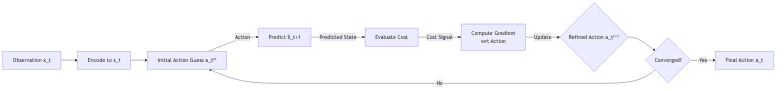
5. Inference-Time Optimization: Thinking on Your Feet

Perhaps JEPA’s most compelling feature is its ability to refine actions at the moment of decision using inference-time optimization in latent space:

5.1 The Optimization Dance

Observe the world $x_t$ , encode it into the current latent state $s_t = \text{Enc}(x_t)$ .
Start with an initial guess for the action $a_t^{(0)}$ (perhaps from a simple policy or just zero).
Iteratively adjust the action using gradient descent on the cost: $a_t^{(i+1)} = a_t^{(i)} - \alpha \nabla_{a} \text{C}(s_t, a_t^{(i)}, \hat{s}_{t+1}^{(i)})$ where $\hat{s}_{t+1}^{(i)} = \text{Pred}(s_t, a_t^{(i)})$ is the predicted future state for the current action guess, and $\alpha$ is a step size. We’re literally asking: “How should I change my action to make the predicted future look better (lower cost)?”
After a few iterations ( $I$ steps), commit to the refined action $a_t = a_t^{(I)}$ .

This leverages the differentiability of the learned components (predictor, cost function) to actively search for better actions in real-time, adapting to the specific situation encoded in $s_t$ .

5.2 How It Stacks Up

This dynamic optimization contrasts sharply with other common AI paradigms:

Approach	Prediction Space	Action Selection	Computational Efficiency	Adaptability
JEPA	Latent space	Inference-time optimization	High (predicts low-dim embeddings)	High (dynamic opt.)
Behavioral Cloning	N/A (direct mapping)	Fixed policy	Very high (simple lookup)	Low (brittle mimicry)
Standard RL (Model-Free)	Value/Policy space	Fixed policy (post-training)	Medium (needs vast training)	Medium (within learned distribution)
Model Predictive Control (MPC)	Observation space	Optimization-based	Low (predicts high-dim observations)	High (dynamic opt.)
Generative World Models	Pixel/observation space	Various (often planning)	Very low (generates full observations)	Medium to high

JEPA hits a sweet spot: adaptability via inference-time optimization, made tractable by operating in the efficient latent space.

6. System Architecture and Information Flow

Visualizing the flow helps understand how the pieces connect:

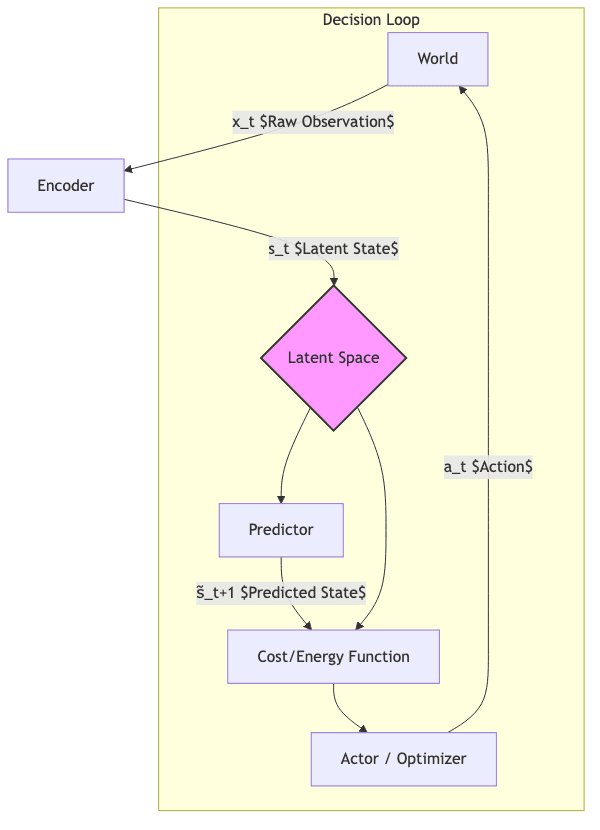
Key pathways emerge:

Perception: World → Encoder → Latent State (Distilling reality)
Prediction: Latent State → Predictor → Future Latent State (Imagining consequences)
Evaluation: Latent State(s) → Cost Module → Cost Signal (Judging futures)
Action: Latent State + Cost → Actor/Optimizer → Action (Choosing based on judgment)
Feedback: Action → World → New Observation → Updated Latent State (Closing the loop)

The entire system is often trainable end-to-end, blending supervised signals (if available) with self-supervised objectives (like making predictions accurate or ensuring costs align with desirable outcomes).

6.1 Mode-1 vs Mode-2 Operation

The two modes visualized:

6.2 Inference-Time Optimization Flow

The action refinement process:

6.3 JEPA’s Place in the AI Menagerie

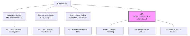
JEPA strategically borrows from multiple paradigms: the representational ambition of generative models (but applied to latent space), the optimization focus of energy-based methods, and the decision-making drive of reinforcement learning, creating something distinct and potentially more efficient.

7. Implementation Example: JEPA in PyTorch

To make this concrete, here’s a conceptual PyTorch implementation showing the core components and their interaction during training and inference. This isn’t production code, but illustrates the structure.

import torch
import torch.nn as nn
import torch.optim as optim
import torch.nn.functional as F

# --------------------------------------------------
# 1. Define Encoder, Predictor, and Cost modules
# --------------------------------------------------

class Encoder(nn.Module):
    """ Encodes observations into latent space """
    def __init__(self, input_dim, latent_dim, hidden_dims=[64, 32]):
        super().__init__()
        layers = []
        dims = [input_dim] + hidden_dims + [latent_dim]
        for i in range(len(dims)-1):
            layers.append(nn.Linear(dims[i], dims[i+1]))
            if i < len(dims)-2: layers.append(nn.ReLU())
        self.network = nn.Sequential(*layers)
    def forward(self, x): return self.network(x)

class Predictor(nn.Module):
    """ Predicts next latent state based on current state and action """
    def __init__(self, latent_dim, action_dim, hidden_dim=64):
        super().__init__()
        self.state_net = nn.Sequential(nn.Linear(latent_dim, hidden_dim), nn.ReLU())
        self.action_net = nn.Sequential(nn.Linear(action_dim, hidden_dim), nn.ReLU())
        self.combined_net = nn.Sequential(
            nn.Linear(hidden_dim * 2, hidden_dim), nn.ReLU(),
            nn.Linear(hidden_dim, latent_dim)
        )
    def forward(self, s, a):
        s_feat = self.state_net(s)
        a_feat = self.action_net(a)
        combined = torch.cat([s_feat, a_feat], dim=1)
        return self.combined_net(combined)

class CostModule(nn.Module):
    """ Assigns scalar cost/energy to latent states (lower is better) """
    def __init__(self, latent_dim, hidden_dim=32):
        super().__init__()
        self.network = nn.Sequential(
            nn.Linear(latent_dim, hidden_dim), nn.ReLU(),
            nn.Linear(hidden_dim, hidden_dim), nn.ReLU(),
            nn.Linear(hidden_dim, 1)
        )
    def forward(self, s): return self.network(s)

class Actor(nn.Module):
    """ Optional explicit policy network (useful for Mode-1 or initial guess) """
    def __init__(self, latent_dim, action_dim, hidden_dim=64):
        super().__init__()
        self.network = nn.Sequential(
            nn.Linear(latent_dim, hidden_dim), nn.ReLU(),
            nn.Linear(hidden_dim, hidden_dim), nn.ReLU(),
            nn.Linear(hidden_dim, action_dim),
            nn.Tanh() # Assuming actions bounded [-1, 1]
        )
    def forward(self, s): return self.network(s)

# --------------------------------------------------
# 2. Training Function (Illustrative)
# --------------------------------------------------

def train_jepa_step(encoder, predictor, cost_fn, optimizer, x_batch, a_batch, x_next_batch, target_states=None):
    """ Single training step for JEPA components """
    s_t = encoder(x_batch)
    with torch.no_grad(): # Target for predictor - stop gradient flow
        s_next_actual = encoder(x_next_batch)

    s_next_pred = predictor(s_t, a_batch)
    pred_loss = F.mse_loss(s_next_pred, s_next_actual) # Make predictions accurate

    # --- Cost Learning (Self-Supervised Example) ---
    # Goal: Make actual observed states lower cost than random/predicted states
    actual_energy = cost_fn(s_next_actual).mean()
    # Energy of predicted states (can also use random noise)
    pred_energy = cost_fn(s_next_pred.detach()).mean()

    # Hinge loss: push actual energy below predicted energy by a margin (e.g., 1.0)
    cost_loss = F.relu(actual_energy - pred_energy + 1.0)
    # Note: More sophisticated contrastive losses are often used here.
    # If target_states (known good states) are available, train cost directly:
    # good_energy = cost_fn(target_states).mean()
    # bad_energy = cost_fn(s_next_pred.detach()).mean() # Or random states
    # cost_loss = F.relu(good_energy - bad_energy + 1.0)
    # --- End Cost Learning ---

    total_loss = pred_loss + 0.5 * cost_loss # Combine losses (weights tunable)

    optimizer.zero_grad()
    total_loss.backward()
    optimizer.step()

    return {'pred_loss': pred_loss.item(), 'cost_loss': cost_loss.item(), 'total_loss': total_loss.item()}

# --------------------------------------------------
# 3. Inference-Time Action Optimization Function
# --------------------------------------------------

def optimize_action(encoder, predictor, cost_fn, x, initial_action, steps=10, lr=0.1):
    """ Refine action at inference time via gradient descent on cost """
    action = initial_action.clone().detach().requires_grad_(True)
    with torch.no_grad():
        s_t = encoder(x) # Encode current state once

    action_optimizer = optim.Adam([action], lr=lr)

    for _ in range(steps):
        s_next_pred = predictor(s_t, action)
        energy = cost_fn(s_next_pred) # Cost of the predicted outcome
        loss = energy.mean() # Minimize this cost

        action_optimizer.zero_grad()
        loss.backward()
        action_optimizer.step()

        # Project action back into valid range if necessary
        with torch.no_grad():
            action.data.clamp_(-1.0, 1.0)

    return action.detach()

# --------------------------------------------------
# 4. System Setup Example
# --------------------------------------------------

def create_jepa_system(input_dim=16, latent_dim=8, action_dim=4):
    """ Instantiate all JEPA components and optimizer """
    encoder = Encoder(input_dim, latent_dim)
    predictor = Predictor(latent_dim, action_dim)
    cost_fn = CostModule(latent_dim)
    actor = Actor(latent_dim, action_dim) # Optional explicit policy

    all_params = list(encoder.parameters()) + list(predictor.parameters()) + \
                 list(cost_fn.parameters()) + list(actor.parameters())
    optimizer = optim.Adam(all_params, lr=3e-4)

    return {'encoder': encoder, 'predictor': predictor, 'cost_fn': cost_fn, 'actor': actor, 'optimizer': optimizer}

# --- Conceptual Execution Loop ---
# env = YourEnvironment()
# jepa = create_jepa_system(env.observation_space.shape[0], latent_dim=16, action_dim=env.action_space.shape[0])
#
# for episode in range(num_episodes):
#     obs = env.reset()
#     for step in range(max_steps):
#         obs_tensor = torch.tensor(obs, dtype=torch.float32).unsqueeze(0) # Add batch dim
#
#         # --- Choose Action ---
#         # Mode-1: Use explicit actor policy
#         # with torch.no_grad():
#         #     latent = jepa['encoder'](obs_tensor)
#         #     action_tensor = jepa['actor'](latent)
#
#         # Mode-2: Optimize action at inference time
#         initial_guess = torch.zeros(1, env.action_space.shape[0]) # Or use actor's output
#         action_tensor = optimize_action(jepa['encoder'], jepa['predictor'], jepa['cost_fn'],
#                                         obs_tensor, initial_guess, steps=20, lr=0.05)
#         # --- End Choose Action ---
#
#         action = action_tensor.squeeze(0).numpy()
#         next_obs, reward, done, info = env.step(action)
#
#         # --- Training ---
#         # Store (obs, action, next_obs) in a replay buffer
#         # Periodically sample batches from buffer and call train_jepa_step(...)
#         # --- End Training ---
#
#         obs = next_obs
#         if done: break

This code sketches out:

The modular nature of JEPA.
The core training loop involving latent prediction loss and cost/energy-based loss (here simplified using a self-supervised hinge loss).
The optimize_action function embodying the inference-time refinement capability.
A conceptual agent loop illustrating how Mode-1 or Mode-2 might be deployed.

It highlights the shift: training focuses on accurate latent prediction and learning a good cost landscape, while decision-making can leverage these learned components dynamically.

8. Applications and Research Frontiers

JEPA’s principles are actively being explored and deployed:

8.1 Computer Vision

Meta AI and others are using JEPA-like self-supervised learning (eg. I-JEPA, V-JEPA). Instead of reconstructing pixels (like masked autoencoders), they predict the embeddings of masked image patches from the embeddings of visible patches. This learns powerful visual representations efficiently, proving effective for downstream tasks like object detection or segmentation without the overhead of pixel generation.

8.2 Robotics and Control

The efficiency of latent prediction makes JEPA attractive for robotics:

Manipulation: Predict effects of grasps or pushes in a compact latent space, avoiding complex physics simulation.
Navigation: Learn abstract maps for efficient path planning.
Sample Efficiency: Potentially learn faster from limited real-world interaction by making better use of each observation through latent prediction.

8.3 Natural Language Processing

While transformers reign supreme, JEPA ideas could influence NLP:

Cross-modal grounding: Aligning language embeddings with visual or auditory latent spaces.
Efficient prediction: Exploring latent-space prediction for tasks where full token-level generation isn’t strictly necessary.

8.4 Multi-Agent Systems

JEPA provides a framework for agents to reason about each other:

Theory of Mind: Predict other agents’ latent states (beliefs, intentions) and actions.
Coordination: Optimize joint actions by predicting collective outcomes in a shared latent space.

9. Situating JEPA in the AI Landscape

JEPA isn’t isolated; it connects to and extends other core AI ideas:

9.1 Relationship to Large Language Models (LLMs)

Modern LLMs like GPT-n operate somewhat analogously:

They maintain internal representations (attention states) summarizing context.
They predict the next token based on this internal state.
They implicitly model only language-relevant aspects of the world.

However, they typically lack JEPA’s explicit energy/cost function and the dedicated inference-time optimization mechanism for action selection (though techniques like beam search or reinforcement learning from human feedback serve related purposes).

9.2 Self-Supervised Learning (SSL)

JEPA heavily relies on SSL techniques to learn its components:

Contrastive Learning: Used to shape the encoder and cost function (e.g., pushing embeddings of similar states closer, dissimilar ones further apart, or making good states low energy).
Masked Prediction: As seen in I-JEPA/V-JEPA, training the predictor by predicting embeddings of masked inputs.

9.3 Model-Based Reinforcement Learning (MBRL)

JEPA shares DNA with MBRL:

The predictor is a form of dynamics model, but operates in latent space.
The cost function acts like a negative reward function or goal specification.
Inference-time optimization resembles planning or Model Predictive Control (MPC).

JEPA’s distinction lies in its explicit rejection of observation-space modeling and its flexible, gradient-based inference-time planning in the learned latent space.

10. Whither JEPA? The Road Ahead

JEPA represents a compelling alternative path for AI development, prioritizing efficient, task-relevant prediction over exhaustive world reconstruction. Key questions remain:

10.1 Scaling Laws

How does JEPA performance scale with model size, data volume, and compute? Does its efficiency advantage over generative models widen or narrow at extreme scales? Understanding these scaling properties is crucial.

10.2 Architectural Hybrids

Can we fruitfully combine JEPA with other architectures? Imagine JEPA-enhanced transformers, or using diffusion models to refine JEPA’s latent predictions occasionally, or hierarchical JEPA systems operating at multiple timescales.

10.3 Theoretical Foundations

We need a deeper theoretical grasp of JEPA: What makes a “good” latent space for prediction and control? What are the convergence guarantees for inference-time optimization? What are the information-theoretic limits of this approach?

10.4 Conclusion: Pragmatism over Purity

Joint Embedding Predictive Architecture offers a potent blend of representation learning, energy-based optimization, and latent dynamics modeling. Its core insight – that predicting abstract representations is often more efficient and effective than predicting raw reality – challenges the prevailing generative paradigm.

By enabling flexible, adaptive decision-making through inference-time optimization within a computationally tractable latent space, JEPA provides a promising direction for building AI systems capable of handling the complexity of the real world without getting bogged down in irrelevant details. It’s a bet on pragmatic efficiency over photorealistic reconstruction, and it might just be the smarter path forward for creating genuinely intelligent agents.