Diffusion Models in AI Image Generation – Part 1: Foundations

Introduction: Yeah, AI Draws Now. So What?

The flood of AI-generated images—DALL·E, Midjourney, Stable Diffusion—is undeniable. Stuff that looked impossible years ago is now commodity, clogging up feeds with uncanny valleys and occasionally brilliant sparks. Underneath much of this pixel-slinging sits a class of algorithms known as diffusion models.

Forget the hype for a second. At their core, denoising diffusion probabilistic models (DDPMs) operate on a surprisingly backward principle: they don’t build images pixel-by-pixel. They start with chaos—pure noise—and learn to meticulously carve coherence out of it. This counter-intuitive approach is what finally cracked the code for generating high-fidelity images with a semblance of control, moving beyond earlier, clunkier methods.

This isn’t magic; it’s a specific kind of engineered intuition. In this two-part series, we’ll dissect it:

Part 1: Foundations (You are here)

Why generating images pixel-by-pixel is a mug’s game.
The core diffusion loop: break it, then fix it.
The key insight: predicting noise is smarter than predicting pixels.
The math that makes the noise prediction work.

Part 2: Applications & Advancements

Getting from text prompts to actual images.
Making it faster: hacks like Latent Consistency Models.
Code glimpses and practical considerations.
Where this noise-wrangling might go next.

By the end, you’ll grasp the ‘why’ behind the current wave of AI image tools – the mechanics beneath the seemingly magical outputs.

The Challenge: How Do You Teach a Machine to Draw?

Before diffusion crashed the party, how did we try to teach machines to generate images? The fundamental problem is immense: creating vast arrays of pixels that aren’t just random garbage, but form structures, obey physics (mostly), and look like something.

The Autoregressive Grind (and Why It Sucks for Images)

One seemingly logical path was to treat image generation like language generation: predict the next element in a sequence. For text, that’s the next word. For images, that’s… the next pixel. This is autoregressive modeling.

How It (Theoretically) Works:

Stare at a blank canvas.
Guess the top-left pixel’s color.
Move one pixel over (or down).
Look at all the pixels you just generated, and guess the next one.
Repeat. A million times.

The Upside:

Conceptually simple, maybe. Borrowed directly from successful language models (like early GPTs).
Can, in theory, model anything given infinite compute.

The Crippling Downsides for Images:

Glacial Pace: A 1024×1024 image demands over a million sequential predictions. Forget interactive speeds; think geological time scales.
Scalability Nightmare: Even predicting patches instead of pixels barely dents the inefficiency.
Myopic Vision: Pixels mostly care about their immediate neighbors. Modeling these tight local dependencies is tricky.
Losing the Plot: The step-by-step nature makes it hard to maintain global coherence. You might get nice textures but end up with a three-eyed dog because the model forgot the big picture halfway through.

Autoregressive image models (like PixelCNN) exist, and they can produce decent results if you’re patient. But for practical, large-scale, fast image generation? It felt like a dead end. We needed a different approach.

The Diffusion Idea: Learn by Breaking, Then Fixing

Diffusion models flipped the script. Instead of building complexity from nothing, they start with complexity (an image) and systematically destroy it, then learn to reverse the destruction. The core question became:

What if you took a perfectly good image, deliberately drowned it in noise, step-by-step, until it was unrecognizable static… and then trained a model to meticulously undo the damage?

This leads to the two phases underpinning diffusion:

The Forward Process: Methodical Vandalism

This part is just a fixed recipe, a predefined way to break images. We don’t learn anything here; we just establish the rules of the game.

Start: Grab a clean image $\mathbf{x}_0$ from your training data.
Corrupt: Add a tiny bit of noise. Then a bit more. Repeat for $T$ steps.
Result: You get a sequence $\mathbf{x}_1, \mathbf{x}_2, ..., \mathbf{x}_T$ , where $\mathbf{x}_T$ is just random noise, indistinguishable from static on an old TV.

The math for each step looks like this:

$\mathbf{x}_t = \sqrt{\alpha_t}\mathbf{x}_{t-1} + \sqrt{1-\alpha_t}\mathbf{\epsilon}$

Where:

$\mathbf{x}_{t-1}$ is the image from the previous step.
$\mathbf{x}_t$ is the slightly noisier image at the current step.
$\alpha_t$ is a number between 0 and 1 that controls how much signal ( $x_{t-1}$ ) vs noise ( $\epsilon$ ) gets mixed in. It usually starts near 1 (keep most signal) and decreases towards 0 (mostly noise).
$\mathbf{\epsilon}$ is just random Gaussian noise, fresh at each step.
The sequence $\alpha_1, ..., \alpha_T$ is the noise schedule – how fast we break the image.

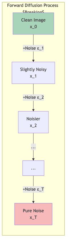
Remember: This forward process is just a setup for training. We never run it when we actually want to generate an image.

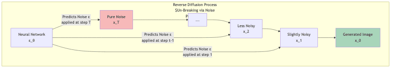
The Reverse Process: Learning to Un-Break

This is where the magic, or rather the learning, happens. We train a neural network to run the process backward:

Start: Generate pure random noise $\mathbf{x}_T$ .
Denoise Step: Feed $\mathbf{x}_T$ into the neural network. Ask it to predict a slightly cleaner version, $\mathbf{x}_{T-1}$ .
Repeat: Feed $\mathbf{x}_{T-1}$ back into the network to get $\mathbf{x}_{T-2}$ , and so on…
Finish: Keep going until you reach $\mathbf{x}_0$ . This final $\mathbf{x}_0$ isn’t the original image (we started with random noise!), but a brand new image synthesized by the model.

The network learns this by seeing countless examples during training: it gets shown a noisy image $\mathbf{x}_t$ and learns what the slightly less noisy $\mathbf{x}_{t-1}$ (or sometimes the original $\mathbf{x}_0$ ) should look like.

The Key Insight: Predict the Noise, Not the Picture

Early attempts had the network try to directly predict the cleaner image $\mathbf{x}_{t-1}$ from the noisy $\mathbf{x}_t$ . This worked okay, but a crucial refinement made diffusion truly effective: train the network to predict the noise ( $\epsilon$ ) that was added, instead of the cleaned image.

Why Predicting Noise is Smarter

Think about the early stages of the reverse process (going from $\mathbf{x}_T$ towards $\mathbf{x}_0$ ). The image is almost pure static. Asking the model “what clean image does this noise hide?” is incredibly hard – there’s almost no signal left.

But asking “what noise pattern was added to get to this state?” is a more constrained, manageable problem:

Clearer Target: The model’s job becomes isolating the structured noise pattern from the underlying (barely visible) signal.
Better Learning Signal: Especially when the image is mostly noise, predicting that noise provides more stable gradients for the network to learn from.
Faster Convergence: Training just works better this way. The models learn more reliably.

The Math Behind Noise Prediction

If you have a model, let’s call it $\epsilon_\theta$ , that takes a noisy image $\mathbf{x}_t$ and the timestep $t$ and predicts the noise $\epsilon$ that was added, you can actually estimate the original clean image $\mathbf{x}_0$ using this prediction:

$\hat{\mathbf{x}}_0 = \frac{\mathbf{x}_t - \sqrt{1 - \alpha_t}\,\epsilon_\theta(\mathbf{x}_t, t)}{\sqrt{\alpha_t}}$

This formula basically says: “Take the noisy image $\mathbf{x}_t$ . Subtract the noise our model predicted ( $\epsilon_\theta$ ), scaled appropriately by how much noise should have been there at step $t$ . What’s left, after scaling back up, is our best guess at the original clean image $\mathbf{x}_0$ .”

The beauty is that the training objective becomes dead simple. We just want our model’s noise prediction $\epsilon_\theta(\mathbf{x}_t, t)$ to be as close as possible to the actual noise $\epsilon$ we added during the forward process simulation:

$\mathcal{L} = \mathbb{E}_{t,\mathbf{x}_0,\epsilon}[||\epsilon - \epsilon_\theta(\mathbf{x}_t, t)||^2]$

Minimize the squared difference between the real noise and the predicted noise. That’s it.

$Reverse Diffusion Process $Un\-Breaking via Noise Prediction$$

Walking Through the Denoising

Think about what the model is doing at different stages:

High Noise (Near $T$ ): The image is mostly static. The model learns to identify broad, low-frequency noise patterns. Getting these right starts to sketch the rough shapes.
Medium Noise (Middle steps): Structures are emerging. The model learns to separate the noise from these nascent forms, refining edges and shapes.
Low Noise (Near $0$ ): The image is almost clean. The model focuses on removing the last subtle noise artifacts, adding fine details and textures.

Code Sketch: The Guts of Training

Here’s a highly simplified PyTorch sketch showing the core training logic:

import torch
import torch.nn as nn
import torch.nn.functional as F

class SimpleDiffusionModel(nn.Module):
    # A stripped-down U-Net placeholder. Real models are much fancier.
    def __init__(self):
        super().__init__()
        self.net = nn.Sequential(
            nn.Conv2d(3, 64, 3, padding=1), # Input: 3-channel noisy image
            nn.ReLU(),
            # ... more layers ... U-Net structure ... attention ... timestep embedding injection ...
            nn.Conv2d(64, 64, 3, padding=1),
            nn.ReLU(),
            nn.Conv2d(64, 3, 3, padding=1)   # Output: 3-channel predicted noise
        )

    def forward(self, x, t):
        # Real models embed 't' and inject it intelligently into the network layers.
        # This is a massive simplification.
        return self.net(x)

# Simplified Training Loop
def train_diffusion(model, dataloader, optimizer, num_timesteps=1000, num_epochs=100):
    # Define the noise schedule (betas -> alphas -> cumulative alphas)
    betas = torch.linspace(0.0001, 0.02, num_timesteps) # Example: linear schedule
    alphas = 1.0 - betas
    alphas_cumprod = torch.cumprod(alphas, dim=0) # ᾱ_t in some papers

    model.train()
    for epoch in range(num_epochs):
        for batch in dataloader: # Assuming batch contains clean images x_0
            optimizer.zero_grad()

            x_0 = batch # Clean images
            batch_size = x_0.size(0)
            device = x_0.device

            # 1. Sample random timesteps for this batch
            t = torch.randint(0, num_timesteps, (batch_size,), device=device).long()

            # 2. Sample random noise ε ~ N(0, I)
            epsilon = torch.randn_like(x_0)

            # 3. Calculate x_t using the closed-form formula (more efficient than iterating)
            #    x_t = sqrt(ᾱ_t) * x_0 + sqrt(1 - ᾱ_t) * ε
            alpha_t_cumprod = alphas_cumprod[t].to(device)
            # Reshape for broadcasting: (batch_size,) -> (batch_size, 1, 1, 1)
            sqrt_alpha_t_cumprod = torch.sqrt(alpha_t_cumprod).view(-1, 1, 1, 1)
            sqrt_one_minus_alpha_t_cumprod = torch.sqrt(1.0 - alpha_t_cumprod).view(-1, 1, 1, 1)

            x_t = sqrt_alpha_t_cumprod * x_0 + sqrt_one_minus_alpha_t_cumprod * epsilon

            # 4. Get the model's noise prediction
            predicted_noise = model(x_t, t) # Pass noisy image and timestep

            # 5. Calculate the loss: Mean Squared Error between actual and predicted noise
            loss = F.mse_loss(predicted_noise, epsilon)

            # 6. Backpropagate and update
            loss.backward()
            optimizer.step()

        print(f"Epoch {epoch}, Loss: {loss.item()}")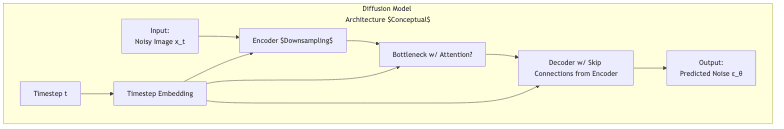

This code snippet captures the essence: pick random times, noise up clean images to those times, ask the model to predict the noise, calculate the error, and adjust the model. Repeat ad nauseam. The real engineering is in the network architecture (often complex U-Nets with attention) and the timestep handling.

The Sampling Speed Problem

Okay, so the theory is neat. But there was a big, practical problem early on: sampling was slow. The original DDPM paper used 1000 steps to generate one image. If each step takes even a fraction of a second, generating batches of images becomes painful.

Steps vs. Quality vs. Speed

Fewer steps means faster generation, but often at the cost of quality. It’s a trade-off:

Sampling Steps	Generation Speed	Image Quality	Feels Like…
1000+	Glacial	Potentially Highest	Academic exercise
100-250	Slow	Very Good	High-end rendering
20-50	Manageable	Good / Great	Sweet Spot Today
4-10	Fast	Often Acceptable	Real-time potential
1-3	Near Instant	Can be rough	Distilled models

Getting from 1000+ steps down to the 20-50 range, without sacrificing too much quality, was crucial for making diffusion models usable. Key developments included:

Better Samplers: Algorithms like DDIM (Denoising Diffusion Implicit Models) realized you didn’t need stochasticity at every step. Making the process deterministic allowed for bigger jumps, drastically cutting steps. DPM-Solver and others pushed this further.
Smarter Noise Schedules: How you define the $\alpha_t$ values matters. Cosine schedules, for instance, often perform better than simple linear ones.
Architecture Gains: Better neural networks just got better at predicting noise accurately, requiring fewer refinement steps.

These combined efforts turned diffusion from a theoretical curiosity into a practical powerhouse.

Code Sketch: DDIM Sampling

Here’s a conceptual look at DDIM sampling, highlighting its deterministic nature compared to the training process:

def sample_ddim(model, shape, num_timesteps=1000, num_ddim_steps=50, eta=0.0):
    """ Sample using DDIM. eta=0 makes it deterministic. """
    device = next(model.parameters()).device
    
    # Noise schedule setup (alphas_cumprod assumed available)
    # ... (same as in training setup) ...

    # Start with pure noise
    x_t = torch.randn(shape, device=device)

    # Define the sampling timesteps (subset of original T)
    # Example: Equally spaced steps in reverse
    times = torch.linspace(num_timesteps - 1, 0, num_ddim_steps + 1).long().to(device)
    
    model.eval()
    with torch.no_grad():
        for i in range(num_ddim_steps):
            # Current timestep t and previous timestep t_prev
            t = times[i].view(-1) # Shape (batch_size,)
            t_prev = times[i+1].view(-1)

            # Get alpha values for current and previous timesteps
            alpha_t = alphas_cumprod[t].view(-1, 1, 1, 1)
            alpha_t_prev = alphas_cumprod[t_prev].view(-1, 1, 1, 1) if t_prev[0] >= 0 else torch.ones_like(alpha_t)

            # 1. Predict the noise ε_θ(x_t, t)
            predicted_noise = model(x_t, t)

            # 2. Estimate the predicted clean image x_0_pred
            x_0_pred = (x_t - torch.sqrt(1. - alpha_t) * predicted_noise) / torch.sqrt(alpha_t)
            # Optional: Clamp x_0_pred to [-1, 1] or similar bounds if needed

            # 3. Calculate the direction pointing to x_t
            pred_dir_xt = torch.sqrt(1. - alpha_t_prev - eta**2) * predicted_noise

            # 4. Calculate x_{t-1} (deterministic update if eta=0)
            x_prev = torch.sqrt(alpha_t_prev) * x_0_pred + pred_dir_xt
            
            # Add stochastic noise if eta > 0
            if eta > 0:
                 sigma_t = eta * torch.sqrt((1. - alpha_t_prev) / (1. - alpha_t) * (1. - alpha_t / alpha_t_prev))
                 noise = torch.randn_like(x_t)
                 x_prev = x_prev + sigma_t * noise
            
            x_t = x_prev # Update for the next iteration

    return x_t # The final generated image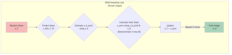

DDIM and similar samplers were game-changers, making high-quality generation feasible in reasonable timeframes.

Conclusion: Laying the Groundwork

So, that’s the bedrock of diffusion models. We’ve seen:

Why the old way (pixel-by-pixel) was painful for images.
The core idea: systematically add noise (forward), then train a model to remove it step-by-step (reverse).
The crucial trick: making the model predict the noise itself is more effective than predicting the clean image directly.
How sampling speed went from a research curiosity to something usable via smarter algorithms like DDIM.

This foundation—starting with noise and iteratively refining towards signal—is why diffusion models exploded onto the scene and now dominate AI image generation. It’s a fundamentally different, and seemingly more effective, way to teach machines about the structure of visual reality.

But this is just the basic engine. How do we steer it with text prompts? How do we make it even faster, potentially real-time? That’s what we’ll tackle in Part 2: Applications & Advancements, looking at text-conditioning, architectural tricks, and techniques like Latent Consistency Models that push the speed limits even further. Stay tuned.

Posted in AI / ML, LLM Intermediate by Rakshit Kalra