One-Step Alignment: Hands-On with ORPO for Fine-Tuning Mistral-7B

Why Chase Yet Another Alignment Method?

The traditional alignment pipeline, whether for RLHF or DPO, was a multi-stage affair. It looked something like this:

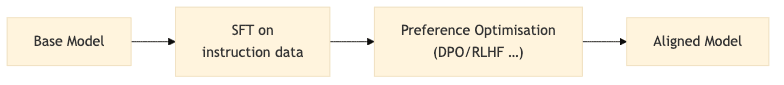
This two-pass approach carries a brutal, practical toll:

A heavier computational tax: You’re paying for two full training runs-two sets of disk I/O, two sets of gradient steps, two validation cycles.
Model sprawl: You’re storing an entire SFT model, often kept as a reference or checkpoint, bloating your storage footprint.
Death by a thousand cuts (in cost): For independent researchers and scrappy startups, the cumulative financial and environmental cost of these redundant stages is a significant drag on innovation.

ORPO’s core insight is that the signal was hiding in plain sight. The logits the model produces already contain enough information to distinguish a preferred response from a rejected one. The challenge wasn’t a lack of information, but a failure of formulation. The goal, then, was to craft a loss function that could simultaneously teach the model to follow instructions and develop a preference for the “better” answer.

Inside the ORPO Loss

To understand how ORPO pulls this off, let’s define our terms:

$x$ is the input prompt.
$y^{+}$ is the chosen (good) completion.
$y^{-}$ is the rejected (bad) completion.
$P_{\theta}(y|x)$ is the probability the model $\theta$ assigns to sequence $y$ given input $x$ .

The classic SFT objective is simply to maximize the log-likelihood of the chosen completion. It’s a one-track mind:

$\mathit{L}_{\textrm{SFT}} = -\log P_{\theta}(y^+|x)$

ORPO grafts onto this a clever penalty based on the odds ratio. This term punishes the model if it doesn’t favor the chosen response over the rejected one. The combined ORPO loss is a monolithic beast:

$\boxed{\; \mathit{L}_{\textrm{ORPO}} = -\log P_{\theta}(y^+|x) \; + \; \lambda \left[ -\log \left( \frac{\textrm{odds}_{\theta}(y^+|x)}{\textrm{odds}_{\theta}(y^-|x)} \right) \right] \; }$

where:

$\textrm{odds}_{\theta}(y|x) = \frac{P_{\theta}(y|x)}{1 - P_{\theta}(y|x)}$
$\lambda$ (the beta parameter in code) is the knob that controls how much we care about the preference penalty versus the basic SFT loss.

Interpretation:

If the model heavily favors $y^+$ over $y^-$ , the odds-ratio term shrinks. The model is rewarded for having good taste.
If the model is ambivalent or, worse, prefers $y^-$ , the odds-ratio term blows up. The model is penalized for its poor judgment.
This forces the model to learn two things at once: how to generate coherent text (the SFT part) and how to distinguish good from bad (the preference part).

Key Points:

This is a sequence-level calculation, not token-by-token. The model judges the whole response.
There’s no sigmoid function here; the penalty is the raw log odds-ratio of the full-sequence probabilities.
$\lambda$ (or beta) is the hyperparameter that balances instruction-following against preference-learning.
There is no ghostly reference model or explicit reward model. Everything is derived from the training model’s own outputs.

This formulation allows ORPO to align a model in a single, unified training phase, killing the need for a separate SFT stage.

How ORPO Stacks Up

Let’s put ORPO in the ring with the other contenders:

Criterion	RLHF	DPO/IPO/KTO	ORPO
Separate SFT model?	✔️ Yes	✔️ Yes	❌ No
Reward model?	✔️ Yes	❌ No	❌ No
GPU memory footprint	Brutal	Tolerable	Sane
Number of training passes	3 (SFT, RM, RL) – Absurd	2 (SFT, PO)	1
Sample efficiency	Good	Good	Might want a larger preference dataset
Empirical quality	★★★★★ (Often SOTA)	★★★★☆ (Strong contender)	★★★★☆* (Punching at the same weight)

* The original ORPO paper shows performance on par with DPO on benchmarks like AlpacaEval and MT-Bench after ~2,000 steps with a batch size of 64. It gets to the same place with less ceremony.

Setting Up the Playground

To get started, you need the right tools. I recommend grabbing the latest versions, especially for TRL, which has native ORPO support.

pip install -q -U bitsandbytes accelerate datasets peft
pip install -q -U git+https://github.com/huggingface/trl.git # TRL nightly for ORPO

Hardware Tips:

FlashAttention-2: If you have a compatible GPU (NVIDIA Ada, Hopper, or anything sm_8x ≥ 80), installing FlashAttention-2 (pip install flash-attn) is not optional. It’s mandatory for your sanity, dramatically cutting training time and memory hunger.
Mixed Precision: Use bfloat16 if your hardware supports it. It’s the sweet spot for speed and stability. Otherwise, fall back to fp16.
GPU Memory: For the recipe below, an NVIDIA RTX 4090 (24 GB) or an A100 (40 GB) is where you stop praying to the OOM killer and start actually training.

From Raw Data to Chat Pairs

For this demonstration, we’ll use the UltraFeedback-binarised dataset. It’s a standard benchmark used for the Zephyr models, and frankly, life is too short to manually process conversation trees for a blog post.

If you insist on using something like OpenAssistant/oasst1, you’ll need to write your own pre-processing script to extract (prompt, chosen, rejected) triplets from the conversation data, then apply the same formatting pipeline below.

Here’s a robust script for data preparation that ensures your tokenizer is ready for battle:

from datasets import load_dataset
from transformers import AutoTokenizer
import multiprocessing as mp

model_id = "mistralai/Mistral-7B-v0.1" # Base model. Instruct version is often better.
tokenizer = AutoTokenizer.from_pretrained(model_id, use_fast=True)

# If your tokenizer throws a fit, it's probably a base model that's dumb about chat.
# Set the template manually. The Instruct versions usually have this pre-set.
if tokenizer.chat_template is None:
    tokenizer.chat_template = "{% for message in messages %}{% if message['role'] == 'user' %}{{ '<s>[INST] ' + message['content'] + ' [/INST]' }}{% elif message['role'] == 'assistant' %}{{ message['content'] + '</s>' }}{% endif %}{% endfor %}"

# If there's no pad token, use the end-of-sentence token. Common practice.
if tokenizer.pad_token is None:
    tokenizer.pad_token = tokenizer.eos_token

# Load and process the dataset
raw_datasets = load_dataset("HuggingFaceH4/ultrafeedback_binarized")
train_dataset_orig = raw_datasets["train_prefs"]
eval_dataset_orig = raw_datasets["test_prefs"]

def format_chat_template(row):
    # row["chosen"] and row["rejected"] are lists of dicts. We need to format them into strings.
    row["chosen"] = tokenizer.apply_chat_template(row["chosen"], tokenize=False)
    row["rejected"] = tokenizer.apply_chat_template(row["rejected"], tokenize=False)
    # The ORPOTrainer expects columns 'prompt', 'chosen', 'rejected'.
    # UltraFeedback provides 'prompt', so we just need to overwrite 'chosen' and 'rejected'.
    return row

num_proc = mp.cpu_count()
train_dataset = train_dataset_orig.map(
    format_chat_template,
    num_proc=num_proc,
)
eval_dataset = eval_dataset_orig.map(
    format_chat_template,
    num_proc=num_proc,
)

Important Note: If you hit an error like tokenizer.chat_template is not set, it’s a clear signal you’re using a base model that knows nothing about chat formats. Use an “instruct” or “chat” variant (e.g., mistralai/Mistral-7B-Instruct-v0.1) which usually has this pre-configured, or set the template manually as shown.

QLoRA + ORPO Implementation

Let’s cut to the chase. Here’s the script to fine-tune Mistral-7B with QLoRA and ORPO, optimized for memory efficiency.

import torch
from transformers import AutoModelForCausalLM, BitsAndBytesConfig
from peft import LoraConfig, prepare_model_for_kbit_training
from trl import ORPOTrainer, ORPOConfig

# model_id and tokenizer are assumed to be loaded from the previous section

# QLoRA configuration for 4-bit quantization
bnb_config = BitsAndBytesConfig(
    load_in_4bit=True,
    bnb_4bit_quant_type="nf4",
    bnb_4bit_compute_dtype=torch.bfloat16 if torch.cuda.is_bf16_supported() else torch.float16,
    bnb_4bit_use_double_quant=True,
)

# Load the model with our QLoRA config
model = AutoModelForCausalLM.from_pretrained(
    model_id,
    quantization_config=bnb_config,
    torch_dtype=torch.bfloat16 if torch.cuda.is_bf16_supported() else torch.float16,
    device_map="auto", # Automatically maps layers to available GPUs
    attn_implementation="flash_attention_2" if torch.cuda.is_bf16_supported() else "sdpa",
)
model = prepare_model_for_kbit_training(model)
model.config.use_cache = False # Critical for training
model.config.pad_token_id = tokenizer.pad_token_id # Set pad token ID

# LoRA configuration
lora_config = LoraConfig(
    r=16,
    lora_alpha=16,
    lora_dropout=0.05,
    bias="none",
    task_type="CAUSAL_LM",
    target_modules=['q_proj', 'k_proj', 'v_proj', 'o_proj',
                    'gate_proj', 'up_proj', 'down_proj']
)

# ORPO configuration
orpo_config = ORPOConfig(
    output_dir="./orpo_mistral7b_results",
    per_device_train_batch_size=2,
    gradient_accumulation_steps=4,       # Effective batch size = 2 * 4 * 8
    learning_rate=8e-6,
    lr_scheduler_type="linear",
    max_steps=500,                       # A short run for demonstration
    beta=0.1,                            # The ORPO λ parameter
    max_length=1024,
    max_prompt_length=512,
    logging_steps=10,
    eval_strategy="steps",
    eval_steps=50,
    save_strategy="steps",
    save_steps=100,
    optim="paged_adamw_8bit",
    warmup_ratio=0.1,
    report_to="tensorboard",
    remove_unused_columns=False,
)

# Initialize the ORPOTrainer
trainer = ORPOTrainer(
    model=model,
    args=orpo_config,
    train_dataset=train_dataset,
    eval_dataset=eval_dataset,
    tokenizer=tokenizer,
    peft_config=lora_config,
)

# Fire it up
trainer.train()

How Long Will It Take?

Training time is not a precise science. Here are some rough estimates based on experience:

GPU Configuration	Estimated Time for 2k steps (batch size 8 effective)	Notes
Google Colab T4 (16GB)	A lesson in futility. Don’t bother.	Memory constrained, painfully slow.
Google Colab L4 / RTX 4090 (24GB)	~30-40 hours	Feasible, but you’ll be watching the clock.
NVIDIA A100 (40GB)	~12-18 hours	The professional’s choice. Fast and stable.

If you only care about the final artifact and not the journey, disable evaluation (eval_strategy="no") to shave off 20-30% of the training time.

Monitoring Progress

During training, the ORPOTrainer spits out several key metrics. Here’s how to read the tea leaves:

train_loss / eval_loss: The combined ORPO loss. This is your main health indicator.
eval_rewards_chosen / eval_rewards_rejected: A proxy for the logits assigned to the chosen/rejected completions. You want the chosen value to climb above the rejected one over time.
eval_rewards_accuracies: The percentage of time the model correctly assigned a higher probability to the chosen response. This is your “taste” metric.
eval_logps_chosen / eval_logps_rejected: The raw average log-probabilities.
eval_margins: The average gap between logps_chosen and logps_rejected. This should trend upwards.

Don’t panic if your preference metrics (accuracy, margins) are flat or even dip at the start. The model has to learn to walk before it can argue. First, it must master generating coherent language (driven by the SFT component of the loss). Once the NLL loss starts to plateau, you’ll see the preference margins climb as the model begins to develop its own judgment.

Scaling Further with GaLore

For those on the bleeding edge of memory efficiency, GaLore (Gradient Low-Rank Projection) offers a path to full-parameter fine-tuning with a memory footprint comparable to LoRA.

To use GaLore, you’d ditch the peft_config and modify the ORPOConfig to use a GaLore-aware optimizer:

# This is a conceptual example. You would not use PEFT/LoRA with GaLore.

orpo_config_galore = ORPOConfig(
    output_dir="./orpo_mistral7b_galore_results",
    per_device_train_batch_size=2,
    gradient_accumulation_steps=4,
    learning_rate=5e-5, # GaLore may require a different learning rate
    max_steps=2000,
    beta=0.1,
    max_length=1024,
    max_prompt_length=512,
    logging_steps=25,
    eval_strategy="steps",
    eval_steps=250,
    save_strategy="steps",
    save_steps=500,
    optim="galore_adamw_8bit_bnb", # The GaLore-specific optimizer
    optim_target_modules=[r".*attn.*", r".*mlp.*"], # Apply GaLore to these modules
    optim_args="rank=128,update_proj_gap=200,scale=0.25", # GaLore hyperparameters
    warmup_ratio=0.1,
    report_to="tensorboard",
    remove_unused_columns=False,
)

# trainer_galore = ORPOTrainer(
#     model=model, # The base, non-PEFT model
#     args=orpo_config_galore,
#     train_dataset=train_dataset,
#     eval_dataset=eval_dataset,
#     tokenizer=tokenizer,
# )
# trainer_galore.train()

The trade-off? GaLore can be slightly slower per step (1.2-1.5x) than QLoRA, but it delivers the performance of a full-parameter tune without the VRAM apocalypse.

Curating Your Own Preference Dataset

Garbage in, garbage out. This axiom is ruthlessly true for preference data. You need a high-quality dataset of (prompt, chosen_response, rejected_response) triplets. Here’s a no-frills recipe for rolling your own:

Generate Candidates: Use a capable model (GPT-3.5, Claude, a strong open-source model) to generate at least two candidate responses for each prompt. Crank up the temperature (0.7-0.9) to get some diversity.
Human Annotation: This is the hard part. Get domain experts or trusted annotators to provide simple binary preferences: which response is better?
Filter the Dross: Discard pairs where annotators can’t agree or where both responses are garbage. You need a clean signal.
Diversity and Scale: Quality trumps quantity, but you still need scale. Aim for at least 10,000 unique prompts for a general-purpose model. For specialized domains, you can start smaller, but the data must be laser-focused.

Choosing the `beta` Hyperparameter

The beta parameter ( $\lambda$ in the math) is the tuning knob that dictates the model’s priorities: should it focus on being a good student (SFT) or a discerning critic (preference)? My experience points to these starting positions:

beta = 0.1 (The Safe Harbor): This is the TRL default for a reason. It’s a sane starting point that prioritizes getting the SFT part right while gently applying preference pressure.
beta = 0.2 to 0.3 (The Accelerator): If your baseline model is already competent, you can increase beta to more aggressively align with your preferences.
beta = 0.5 or higher (Here Be Dragons): High values can force strong preference alignment but risk “over-optimization,” where the model becomes a sycophant for your specific preferences, losing its general helpfulness or fluency. Tread carefully.
Annealing beta (The Pro Move): In highly constrained domains (e.g., legal or medical AI), you can start beta high (0.2–0.3) to teach the rules, then gradually anneal it to a lower value (0.05–0.1) in the final phase of training to polish its general capabilities.

Don’t guess. Validate. Test your beta on a held-out set that measures both preference accuracy and overall quality. Anything else is malpractice.

Conclusion

ORPO represents a compelling simplification of the LLM alignment pipeline, a sign of maturity in the field. By collapsing the SFT and preference stages into one, it scraps the baroque, multi-stage rituals of the past for something more integrated, efficient, and philosophically sound.

I encourage you to experiment. The tools are getting simpler. The excuses for not building are getting thinner. I’m curious to hear how your own results stack up.