Llama 4 and the 10 Million-Token Context: An Engineering Reality Check

Key Takeaways

10M tokens is not a magic wand for comprehension. While you can technically feed a model a massive prompt, the economic and operational physics are unforgiving.
The true bottleneck isn’t model size; it’s the colossal memory appetite of the KV-cache. For a model like Llama 4-Scout-17B, the KV-cache for a 10 million-token sequence at 16-bit precision demands a staggering 1.23 TB of VRAM.
Architectural cleverness-Grouped-Query Attention (GQA), advanced RoPE-is what makes these numbers even theoretically plausible. These are the hacks that keep scaling laws from blowing up quadratically.
Survival tactics against the memory wall include aggressive quantization (FP8/4-bit), tensor parallelism, or the devil’s bargain of cache recomputation. Each choice has a cost in accuracy or latency.
For most real-world problems, Retrieval-Augmented Generation (RAG) remains the pragmatic, and often superior, choice. This is unlikely to change anytime soon.

Why Even Talk About 10 Million Tokens?

When Meta floated the idea of a 10 million-token context window for a preview model like Llama 4-Scout, the usual hype cycle kicked in. The headlines bloomed, some proclaiming the imminent death of Retrieval-Augmented Generation (RAG). The allure is obvious: if a model can “see” an entire library in a single glance, why bother with the messy mechanics of a retrieval system?

This is a seductive narrative. But as an engineer who lives in the trenches of deploying these systems, I know that context length is just one vertex of an iron triangle. The other two, equally brutal, vertices are latency and cost. Push one too far-like ballooning the context window to planetary scale-and the entire structure collapses into something practically useless.

Here, we will cut through the noise and look at the cold, hard numbers. The memory footprints, the GPU stacks, the dollar signs. I’ll also lay out the techniques we use in the lab to tame these monster contexts, offering a dose of pragmatism against the prevailing speculation.

From Formula to Terabytes: Sizing the KV-Cache

Understanding the KV-Cache in GQA Models

The mechanics of autoregressive generation are unforgiving. To produce text token by token, each new token must attend to every single token that came before it. To avoid recomputing the Key (K) and Value (V) vectors for the entire history at every single step-an act of computational suicide-inference engines cache these vectors in GPU memory. This is the KV-cache. It is the beast you must feed.

For models that use Grouped-Query Attention (GQA), the KV-cache size per layer is a direct function of the sequence length and model architecture:

$M_{\textrm{KV/layer}} = 2 \times s \times b \times n_{\textrm{kv\_{h}eads}} \times d_{\textrm{head}}$

Where:

$s$ : sequence length (number of tokens)
$b$ : batch size
$n_{\textrm{kv\_{h}eads}}$ : number of KV heads in GQA. This is less than or equal to the number of query heads.
$d_{\textrm{head}}$ : dimension of each attention head.

The total KV-cache memory for all layers ( $L$ ) in Gigabytes (GB), assuming a given bitwidth for storing each value (e.g., 16 bits for FP16/BF16), is:

$M_{\textrm{KV (total)}} = L \times (2 \times s \times b \times n_{\textrm{kv\_{h}eads}} \times d_{\textrm{head}}) \times \frac{\textrm{bitwidth}}{8 \times 10^9} \quad [\textrm{GB}]$

For specific architectures like the Llama 4-Scout-17B parameters we’re using, relationships exist that simplify the formula. It turns out that the term $n_{\textrm{kv\_{h}eads}} \times d_{\textrm{head}}$ can be expressed as $\frac{d_{\textrm{model}}}{n_{\textrm{kv\_{h}eads}}}$ , where $d_{\textrm{model}}$ is the model’s hidden size.

This gives us a cleaner working formula for Scout-17B:

$M_{\textrm{KV}} = L \times s \times b \times 2 \times \left(\frac{\textrm{hidden\_{s}ize}}{\textrm{num\_{k}v\_{h}eads}}\right) \times \frac{\textrm{bitwidth}}{8 \times 10^9} \quad [\textrm{GB}]$

Let’s define the parameters for our example, the hypothetical Llama 4-Scout-17B:

Symbol	Meaning	Scout-17B Value
$L$	# transformer layers	48
$s$	sequence length (tokens)	10,000,000 (10M)
hidden_{s}ize	model hidden dimension	5120
$b$	batch size	1
num_{k}v_{h}eads	# KV heads	8
bitwidth	bits per cache element	16 (for FP16/BF16)

For Scout-17B, the term (hidden_size / num_kv_heads) is 5120 / 8 = 640.

Rule of thumb: For a model like Llama 4-Scout-17B at 16-bit precision, burn this into your brain: you need roughly 1GB of KV-cache for every 8,000 tokens.

Plugging in the Numbers for Llama 4-Scout-17B

Let’s calculate the KV-cache for Scout-17B with a 10 million token sequence, a batch size of one, and 16-bit precision.

$M_{\textrm{KV}} = 48 \times 10,000,000 \times 1 \times 2 \times \left(\frac{5120}{8}\right) \times \frac{16}{8 \times 10^9}$ $M_{\textrm{KV}} = 48 \times 10,000,000 \times 2 \times 640 \times \frac{2}{10^9}$ $M_{\textrm{KV}} = 48 \times 10^7 \times 2 \times 640 \times 2 \times 10^{-9}$ $M_{\textrm{KV}} = 1,228,800,000,000 \times 10^{-9} \textrm{ GB}$ $M_{\textrm{KV}} \approx 1228.8 \textrm{ GB} \approx \mathbf{1.23 \textrm{ TB}}$

And that 1.23 TB? That’s just the price of admission for the KV-cache. The model weights themselves, a mere ~34 GB for a 17B parameter model at FP16, are a rounding error in comparison. Add runtime overheads, and you begin to grasp the scale of the problem.

A Hands-On Estimator

To make this less abstract and more visceral, here is a simple Python script. It uses the simplified formula to show how the memory bill explodes.

# kv_memory_estimator.py
from dataclasses import dataclass

@dataclass
class KVSpec:
    layers: int           # L, Number of transformer layers
    hidden: int           # h, Model's hidden size (d_model)
    # For models like Scout-17B where d_model / num_kv_heads_actual = num_kv_heads_actual * head_dim,
    # this 'kv_heads' parameter refers to num_kv_heads_actual.
    # The term (self.hidden // self.kv_heads) then correctly calculates num_kv_heads_actual * head_dim.
    kv_heads: int         # g, Number of KV heads (actual)
    bitwidth: int = 16    # Bitwidth for cache elements (e.g., 16 for FP16, 8 for FP8)
    batch: int = 1        # b, Batch size

    def estimate_gqa_kv_cache(self, seq_len: int) -> float:
        """
        Estimates KV-cache size in GB for GQA models like Llama 4-Scout-17B.
        The term (self.hidden // self.kv_heads) represents (d_model / num_kv_heads_actual),
        which for Scout-17B's specific GQA configuration equals (num_kv_heads_actual * head_dim).
        """
        bytes_per_element = self.bitwidth / 8
        
        # Factor representing (num_kv_heads * head_dim)
        # For Scout-17B: (5120 // 8) = 640. (This equals 8 KV heads * 80 head_dim)
        effective_dim_per_layer_kv = (self.hidden // self.kv_heads)
        
        # Total bytes for K and V tensors across all layers
        total_bytes = 2 * self.layers * seq_len * self.batch * effective_dim_per_layer_kv * bytes_per_element
        return round(total_bytes / 1e9, 3)  # Convert to GB

if __name__ == "__main__":
    # Parameters for Llama 4-Scout-17B (hypothetical)
    # L=48, hidden_size=5120, num_kv_heads=8 (actual), head_dim=80
    # num_query_heads = 64 (so GQA ratio is 64/8 = 8)
    scout_params = KVSpec(layers=48, hidden=5120, kv_heads=8) # kv_heads here is actual num_kv_heads

    print("KV-Cache Memory Estimates for Llama 4-Scout-17B (FP16):")
    for tokens in (1_000, 10_000, 1_000_000, 10_000_000):
        gb_needed = scout_params.estimate_gqa_kv_cache(tokens)
        print(f"{tokens:>12,} tokens → {gb_needed:7.3f} GB")

    print("\nKV-Cache Memory Estimates for Llama 4-Scout-17B (FP8):")
    scout_params_fp8 = KVSpec(layers=48, hidden=5120, kv_heads=8, bitwidth=8)
    for tokens in (1_000, 10_000, 1_000_000, 10_000_000):
        gb_needed = scout_params_fp8.estimate_gqa_kv_cache(tokens)
        print(f"{tokens:>12,} tokens → {gb_needed:7.3f} GB")

The script’s output tells a clear story:

KV-Cache Memory Estimates for Llama 4-Scout-17B (FP16):
       1,000 tokens →   0.123 GB
      10,000 tokens →   1.229 GB
   1,000,000 tokens → 122.880 GB
  10,000,000 tokens → 1228.800 GB

KV-Cache Memory Estimates for Llama 4-Scout-17B (FP8):
       1,000 tokens →   0.061 GB
      10,000 tokens →   0.614 GB
   1,000,000 tokens →  61.440 GB
  10,000,000 tokens → 614.400 GB

The math is simple and brutal. Switching the cache to 8-bit precision halves the memory bill. An obvious first move.

GPUs, Nodes & Dollars: The Hardware Reality

These abstract terabytes translate into a very concrete, very expensive pile of silicon. This is what it takes to field this capability, based on today’s high-end hardware and spot pricing that changes by the hour.

Configuration	Total GPU Mem (GB)	Est. Max Context (Scout-17B, FP16 KV)†	Approx. Hourly Cost‡
1x H100 Node (8 GPUs)	8 x 80GB = 640 GB	≈ 4.5M tokens	$28
1x H200 Node (8 GPUs)	8 x 141GB = 1128 GB	≈ 8M tokens	$47
Multi-Node: 32x H100-80GB	32 x 80GB = 2560 GB	≈ 10M tokens (fits KV + model)	≈ $115
Multi-Node: 32x A100-80GB	32 x 80GB = 2560 GB	≈ 10M tokens (slower inference)	≈ $72

† Maximum context estimates account for the KV-cache (1.23TB for 10M tokens at FP16), model weights (~34GB), and operational overhead. My own estimations are grounded in the memory appetite of systems like vLLM. Your mileage will vary. ‡ Spot pricing from providers like RunPod or Lambda Labs is a moving target. These are April 2025 snapshots.

To serve a 10 million token context for Scout-17B at FP16 precision, you are looking at a cluster of at least four 8xH100 nodes-32 GPUs in total-just to get in the game.

Making It Fit: Strategies for Optimization

If 1.23 TB for the KV-cache alone feels like an insurmountable wall, it’s because it often is. But we have weapons to fight back.

FP8 KV-Cache

As the numbers show, switching the KV-cache to FP8 precision (e.g., via --kv-cache-dtype fp8 in vLLM) cuts the memory requirement in half. For many tasks, the hit to model quality is negligible. This is the first, most obvious lever to pull.

Aggressive Quantization (4-bit, 2-bit)

Frameworks like HQQ (Half-Quadratic Quantization) are pushing quantization to the breaking point, down to 4-bit and even 2-bit. Below 4-bit, accuracy degradation can become severe, but for certain retrieval or summarization tasks over vast contexts, the trade-off might be worth it.

Cache-Free Recomputation (Attention Sinks, StreamingLLM)

Some approaches try to sidestep the problem by not storing the entire KV-cache. Techniques like “attention sinks” (StreamingLLM) cache only a small window of recent tokens plus a few initial “anchor” tokens. This is a devil’s bargain: you trade VRAM for time, paying a severe latency penalty to recompute any historical token outside the cache. It minimizes memory but cripples performance for tasks needing non-local attention.

Tensor and Pipeline Parallelism

When the memory required exceeds a single node, distribution is the only answer. Tensor Parallelism splits individual model layers across GPUs, while Pipeline Parallelism puts different layers on different GPUs. The viability of this lives and dies by the interconnect bandwidth (NVLink, InfiniBand) and the intelligence of the underlying framework (DeepSpeed, Megatron-LM).

Does This Kill RAG?

So, is this the death knell for RAG? The narrative is seductive, but wrong. Long contexts are powerful, but they solve a different class of problem. They shine when:

The interaction is inherently streaming and stateful, like a very long conversation where retrieving and re-injecting context at every turn is clumsy and inefficient.
The task demands holistic, order-dependent, global reasoning across the entire text. Think analyzing a huge codebase for subtle architectural flaws, grasping the full narrative arc of a novel, or finding contradictions in a thousand-page legal discovery.
The latency of reasoning is already the dominant cost, making the addition of an external retrieval step a net loss.

RAG systems, powered by brutally efficient vector search (see Pinecone or Elasticsearch), will continue to dominate when:

Latency is paramount. A P99 vector search is measured in milliseconds. Full attention over 10M tokens is orders of magnitude slower, especially on the first “prefill” pass.
The required information is sparse. If the answer is in two paragraphs of a million-page library, it is absurdly inefficient to force the LLM to read the entire library. It’s better to find the paragraphs.
Freshness, traceability, and factuality are non-negotiable. RAG allows you to update your knowledge base on the fly and provides direct citations to source material. A monolithic context is an opaque, un-updatable black box.

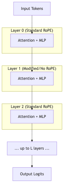
How Llama 4 Might Stretch Position Embeddings: iRoPE

The magic that even allows us to contemplate these context lengths isn’t brute force; it’s architectural cleverness. Traditional Rotary Position Embeddings (RoPE), as detailed in the original paper, are brilliant but struggle when extrapolating far beyond their training length.

Llama 4 almost certainly uses a refinement. A likely candidate is a strategy like iRoPE (Interleaved RoPE), which modulates how positional information is applied across different layers. Some layers might use standard RoPE, others a modified version, and some might skip it entirely. This “interleaving” helps the positional signal propagate over vast distances without degrading.

This is the ghost in the machine that makes the headline number possible.

When paired with a training regimen that gradually increases context length, the architecture can accept inputs up to 10 million tokens. But whether it can truly reason across that chasm is the billion-dollar question. Its effective intelligence at those extreme, unseen lengths requires brutal, honest evaluation, not just faith in extrapolation.

Closing Thoughts

The ambition behind 10 million-token context windows is undeniable. The prospect of an LLM ingesting and reasoning over entire codebases or libraries in a single pass is a powerful vision. It promises to eliminate entire categories of complex data chunking and management.

Yet, as we’ve seen, the engineering reality bites hard:

Terabyte-scale GPU clusters are the baseline requirement, not the exception.
Even with optimizations like FlashAttention-2, the latency to process 10 million tokens is substantial, especially for the initial prefill.
Models are trained on contexts far shorter than what they advertise. Extrapolating to 10M from a 256k or 2M training context is a leap of faith built on architectural tricks. The quality at the edges is not guaranteed.

So, my rule of thumb remains unchanged:

Use large contexts for conversational continuity and deep analysis of data-in-hand. Use RAG for efficient, traceable integration of broad domain knowledge.

When the calculus of cost, latency, and true reasoning capability shifts-perhaps through new breakthroughs in sparse attention or a fundamental change in the economics of memory-I will be the first to reconsider. Until then, if you plan to enter the world of mega-contexts, bring a lot of hardware and a healthy dose of skepticism.